Pandas DataFrame
Pandas is an open-source Python library that provides high-performance, easy-to-use data structures and data analysis tools. Among its core offerings, the Pandas DataFrame is one of the most important data structures in Pandas. It is essentially a two-dimensional labeled data structure with columns of potentially different types of data. In this article, we will explore the various functionalities of the Pandas DataFrame with comprehensive examples.
Pandas DataFrame Recommended Articles
- pandas dataframe add column
- pandas dataframe append
- pandas dataframe apply
- pandas dataframe filter
- pandas dataframe filter by column value
- pandas dataframe from dict
- pandas dataframe from list
- pandas dataframe groupby
- pandas dataframe loc and iloc
- pandas dataframe loc column
- pandas dataframe loc
- pandas dataframe loc condition
- pandas dataframe loc 2 conditions
- pandas dataframe loc example
- pandas dataframe loc datetime
- pandas dataframe loc iloc
- pandas dataframe loc in list
- pandas dataframe loc keyerror
- pandas dataframe loc multiindex
- pandas dataframe loc multiple columns
- pandas dataframe loc multiple conditions
- pandas dataframe loc or operator
- pandas dataframe loc two conditions
- pandas dataframe loc vs iloc
- pandas dataframe loc with multiple conditions
- pandas dataframe merge
- pandas dataframe rename column
- pandas dataframe to csv
- pandas dataframe to list
1. Creating a Pandas DataFrame
One of the most basic operations when working with Pandas is creating a Pandas DataFrame. You can create a Pandas DataFrame from various data sources like lists, dictionaries, and even from external data files.
Example 1: Creating a Pandas DataFrame from a List
import pandas as pd

data = [['Alex', 10], ['Bob', 12], ['Clarke', 13]]
df = pd.DataFrame(data, columns=['Name', 'Age'])
print(df)
Output:

Example 2: Creating a Pandas DataFrame from a Dictionary
import pandas as pd

data = {'Name': ['Tom', 'Jack', 'Steve', 'Ricky'],
        'Age': [28, 34, 29, 42]}
df = pd.DataFrame(data)
print(df)
Output:

2. Reading and Writing Data in Pandas DataFrame
Pandas supports reading from and writing to different data formats including CSV, Excel, SQL databases, and more.
Example 3: Reading Data from CSV
import pandas as pd

df = pd.read_csv('pandasdataframe.com_data.csv')
print(df)
Example 4: Writing Data to Excel
import pandas as pd

df = pd.DataFrame({'Data': [10, 20, 30, 20, 15, 30, 45]})
df.to_excel('pandasdataframe.com_output.xlsx', index=False)
3. Data Selection, Addition, and Deletion in Pandas DataFrame
Manipulating data is central to using Pandas effectively. You can select, add, or delete data in a Pandas DataFrame.
Example 5: Selecting Data by Column in Pandas DataFrame
import pandas as pd

data = {'Name': ['Tom', 'Jerry', 'Mickey', 'Donald'],
        'Age': [25, 30, 35, 40]}
df = pd.DataFrame(data)
print(df['Name'])
Output:

Example 6: Adding a New Column in Pandas DataFrame
import pandas as pd

df = pd.DataFrame({'Name': ['Tom', 'Jack', 'Steve', 'Ricky'],
                   'Age': [28, 34, 29, 42]})
df['Salary'] = [1000, 1500, 1200, 1800]
print(df)
Output:

Example 7: Deleting a Column in Pandas DataFrame
import pandas as pd

data = {'Name': ['Tom', 'Jerry', 'Mickey', 'Donald'],
        'Age': [25, 30, 35, 40]}
df = pd.DataFrame(data)
df.drop('Age', axis=1, inplace=True)
print(df)
Output:

4. Handling Missing Data in Pandas DataFrame
Handling missing data is another critical part of data analysis. Pandas provides several methods to deal with missing data in DataFrames.
Example 8: Filling Missing Data in Pandas DataFrame
import pandas as pd
import numpy as np

df = pd.DataFrame({'First Score': [100, 90, np.nan, 95],
                   'Second Score': [30, 45, 56, np.nan],
                   'Third Score': [np.nan, 40, 80, 98]})
df.fillna(0, inplace=True)
print(df)
Output:

Example 9: Dropping Rows with Missing Data in Pandas DataFrame
import pandas as pd
import numpy as np

df = pd.DataFrame({'First Score': [100, 90, np.nan, 95],
                   'Second Score': [30, 45, 56, np.nan],
                   'Third Score': [np.nan, 40, 80, 98]})
df.dropna(inplace=True)
print(df)
Output:

5. Pandas DataFrame Operations
Pandas DataFrames support a variety of operations that can be very useful in data analysis and manipulation.
Example 10: Performing Arithmetic Operations in Pandas DataFrame
import pandas as pd

df = pd.DataFrame({
    'A': [14, 4, 5, 4, 1],
    'B': [5, 2, 54, 3, 2],
    'C': [20, 20, 7, 3, 8],
    'D': [14, 3, 6, 2, 6]})
df['A'] = df['A'] + 10
print(df)
Output:

Example 11: Applying Functions to Data in Pandas DataFrame
import pandas as pd

df = pd.DataFrame({
    'A': [14, 4, 5, 4, 1],
    'B': [5, 2, 54, 3, 2],
    'C': [20, 20, 7, 3, 8],
    'D': [14, 3, 6, 2, 6]})
df = df.apply(lambda x: x + 10)
print(df)
Output:

6. Grouping and Aggregating Data in Pandas DataFrame
Grouping and aggregating data is essential when you are dealing with large datasets or when you need to perform operations on categorized data.
Example 12: Grouping Data by Column in Pandas DataFrame
import pandas as pd

data = {'Company': ['Google', 'Google', 'Microsoft', 'Microsoft', 'Facebook', 'Facebook'],
        'Person': ['Sam', 'Charlie', 'Amy', 'Vanessa', 'Carl', 'Sarah'],
        'Sales': [200, 120, 340, 124, 243, 350]}
df = pd.DataFrame(data)
grouped_df = df.groupby('Company')
print(grouped_df.mean())
Example 13: Aggregating Data Using Multiple Functions in Pandas DataFrame
import pandas as pd

data = {'Company': ['Google', 'Google', 'Microsoft', 'Microsoft', 'Facebook', 'Facebook'],
        'Person': ['Sam', 'Charlie', 'Amy', 'Vanessa', 'Carl', 'Sarah'],
        'Sales': [200, 120, 340, 124, 243, 350]}
df = pd.DataFrame(data)
grouped_df = df.groupby('Company').agg({'Sales': ['mean', 'sum']})
print(grouped_df)
Output:

7. Merging, Joining, and Concatenating in Pandas DataFrame
Combining multiple datasets is a common task in data analysis. Pandas provides multiple ways to merge, join, or concatenate DataFrames.
Example 14: Concatenating Pandas DataFrames
import pandas as pd

df1 = pd.DataFrame({
    'A': ['A0', 'A1', 'A2', 'A3'],
    'B': ['B0', 'B1', 'B2', 'B3'],
    'C': ['C0', 'C1', 'C2', 'C3'],
    'D': ['D0', 'D1', 'D2', 'D3']},
    index=[0, 1, 2, 3])

df2 = pd.DataFrame({
    'A': ['A4', 'A5', 'A6', 'A7'],
    'B': ['B4', 'B5', 'B6', 'B7'],
    'C': ['C4', 'C5', 'C6', 'C7'],
    'D': ['D4', 'D5', 'D6', 'D7']},
    index=[4, 5, 6, 7])

result = pd.concat([df1, df2])
print(result)
Output:

Example 15: Merging Pandas DataFrames on Key
import pandas as pd

left = pd.DataFrame({
    'key': ['K0', 'K1', 'K2', 'K3'],
    'A': ['A0', 'A1', 'A2', 'A3'],
    'B': ['B0', 'B1', 'B2', 'B3']})

right = pd.DataFrame({
    'key': ['K0', 'K1', 'K2', 'K3'],
    'C': ['C0', 'C1', 'C2', 'C3'],
    'D': ['D0', 'D1', 'D2', 'D3']})

result = pd.merge(left, right, on='key')
print(result)
Output:

Example 16: Joining Pandas DataFrames
import pandas as pd

left = pd.DataFrame({
    'A': ['A0', 'A1', 'A2'],
    'B': ['B0', 'B1', 'B2']},
    index=['K0', 'K1', 'K2'])

right = pd.DataFrame({
    'C': ['C0', 'C1', 'C2'],
    'D': ['D0', 'D1', 'D2']},
    index=['K0', 'K2', 'K3'])

result = left.join(right)
print(result)
Output:

8. Advanced Pandas DataFrame Operations
As you become more familiar with Pandas, you’ll encounter situations that require advanced operations such as pivoting, melting, and applying custom transformations.
Example 17: Pivoting Pandas DataFrames
Pivoting a table is a common operation in data analysis that involves transforming data from long format to wide format.
import pandas as pd

data = {'Date': ['2023-01-01', '2023-01-01', '2023-01-02', '2023-01-02'],
        'Type': ['A', 'B', 'A', 'B'],
        'Value': [100, 200, 300, 400]}
df = pd.DataFrame(data)
pivot_df = df.pivot(index='Date', columns='Type', values='Value')
print(pivot_df)
Output:

Example 18: Melting Pandas DataFrames
Melting is the opposite of pivoting and changes the Pandas DataFrame from wide format to long format.
import pandas as pd

df = pd.DataFrame({
    'Date': ['2023-01-01', '2023-01-02'],
    'A': [100, 300],
    'B': [200, 400]})
melted_df = pd.melt(df, id_vars=['Date'], value_vars=['A', 'B'])
print(melted_df)
Output:

Example 19: Applying Custom Transformations Using applymap
The applymap function allows you to apply a function to every single element in the Pandas DataFrame.
import pandas as pd

df = pd.DataFrame({
    'A': [1, 2, 3],
    'B': [4, 5, 6],
    'C': [7, 8, 9]})
df = df.applymap(lambda x: x**2)
print(df)
Example 20: Filtering Data in Pandas DataFrame
Filtering allows you to select a subset of rows that meet certain criteria.
import pandas as pd

df = pd.DataFrame({
    'Name': ['Tom', 'Nick', 'Krish', 'Jack'],
    'Age': [20, 21, 19, 18]})
filtered_df = df[df['Age'] > 19]
print(filtered_df)
Output:

9. Time Series Data
Pandas is particularly strong in working with time series data. You can perform various operations specific to time series data like resampling, time shifts, and window functions.
Example 21: Resampling Time Series Data in Pandas DataFrame
Resampling involves changing the frequency of your time series observations.
import pandas as pd
import numpy as np

idx = pd.date_range('20230101', periods=60, freq='D')
ts = pd.Series(range(len(idx)), index=idx)
resampled_ts = ts.resample('M').mean()
print(resampled_ts)
Example 22: Time Shifting
Time shifting lets you move data forward or backward in time.
import pandas as pd

df = pd.DataFrame({
    'sales': [3, 5, 2, 6],
    'signups': [5, 5, 6, 12],
    'visits': [20, 42, 28, 62]},
    index=pd.date_range(start='2023-01-01', periods=4))
df_shifted = df.shift(1)
print(df_shifted)
Output:

Example 23: Window Functions
Window functions are useful for calculating rolling statistics.
import pandas as pd

s = pd.Series([1, 2, 3, 4, 5, 6, 7, 8, 9, 10])
rolling_mean = s.rolling(window=3).mean()
print(rolling_mean)
Output:

Pandas DataFrame Conclusion
Pandas DataFrame is a powerful tool for data manipulation and analysis. By understanding how to effectively use its various functionalities, you can perform a wide range of data analysis tasks more efficiently. This article has provided a comprehensive overview of the key features of Pandas DataFrame along with practical examples to help you get started with data analysis in Python. Whether you are dealing with small datasets or large, structured or unstructured data, Pandas offers the functionality you need to clean, transform, and analyze your data.