Pandas Correlation Between Multiple Columns

Pandas Correlation Between Multiple Columns

Correlation analysis is a vital statistical tool that helps in determining the degree to which two or more variables fluctuate with respect to each other. In data science, understanding the correlation between multiple columns in datasets can provide insights into the relationships between features, which is crucial for feature selection, data preprocessing, and building predictive models.

Pandas, a powerful data manipulation library in Python, offers several functions to compute correlations between multiple columns easily. This article will explore how to use Pandas to calculate correlations and interpret the results, with a focus on practical examples.

Understanding Correlation

Correlation coefficients range from -1 to 1. A coefficient close to 1 implies a strong positive correlation: as one variable increases, the other variable tends to also increase. A coefficient close to -1 implies a strong negative correlation: as one variable increases, the other variable tends to decrease. A coefficient around 0 implies no linear correlation between the variables.

Types of Correlation Coefficients

1. Pearson: Measures linear correlation between datasets.
2. Spearman: Used when the data is not normally distributed or the relationship is not linear.
3. Kendall: Used for data with a natural ordinal classification.

Setting Up Your Environment

Before diving into the examples, ensure you have the Pandas library installed in your Python environment:

pip install pandas

Example 1: Basic Correlation Matrix

This example demonstrates how to create a basic correlation matrix between multiple columns in a DataFrame.

import pandas as pd

# Sample data
data = {
    'A': [1, 2, 3, 4, 5],
    'B': [5, 4, 3, 2, 1],
    'C': [2, 3, 2, 3, 2]
}
df = pd.DataFrame(data)

# Compute the Pearson correlation matrix
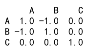
correlation_matrix = df.corr()
print(correlation_matrix)

Output:

Example 2: Spearman Correlation

This example shows how to compute the Spearman correlation coefficient, which does not assume a normal distribution of the data.

import pandas as pd

# Sample data
data = {
    'A': [1, 2, 3, 4, 5],
    'B': [5, 4, 3, 2, 1],
    'C': [2, 3, 2, 3, 2]
}
df = pd.DataFrame(data)

# Compute the Spearman correlation
spearman_corr = df.corr(method='spearman')
print(spearman_corr)

Output:

Example 3: Kendall Correlation

This example calculates the Kendall correlation coefficient, which is particularly useful for data with an ordinal classification.

import pandas as pd

# Sample data
data = {
    'A': [1, 2, 3, 4, 5],
    'B': [5, 4, 3, 2, 1],
    'C': [2, 3, 2, 3, 2]
}
df = pd.DataFrame(data)

# Compute the Kendall correlation
kendall_corr = df.corr(method='kendall')
print(kendall_corr)

Output:

Example 4: Correlation with Non-Numeric Data

Handling non-numeric data requires encoding before correlation analysis. This example demonstrates handling categorical data.

import pandas as pd

# Sample data
data = {
    'A': [1, 2, 3, 4, 5],
    'B': ['low', 'low', 'high', 'high', 'medium'],
}
df = pd.DataFrame(data)

# Convert categorical data to numeric
df['B'] = df['B'].astype('category').cat.codes

# Compute the Pearson correlation
correlation_matrix = df.corr()
print(correlation_matrix)

Output:

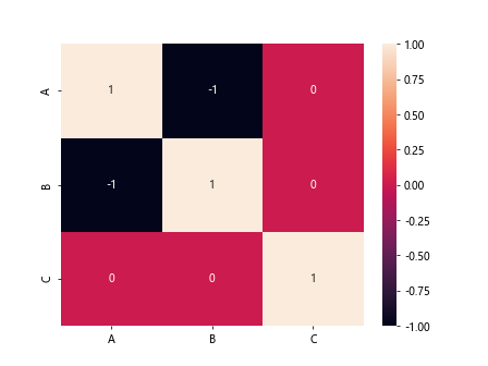
Example 5: Heatmap of Correlation Matrix

Visualizing the correlation matrix using a heatmap can be more insightful. This example requires the seaborn library for plotting.

import pandas as pd
import seaborn as sns
import matplotlib.pyplot as plt

# Sample data
data = {
    'A': [1, 2, 3, 4, 5],
    'B': [5, 4, 3, 2, 1],
    'C': [2, 3, 2, 3, 2]
}
df = pd.DataFrame(data)

# Compute the Pearson correlation matrix
correlation_matrix = df.corr()

# Create a heatmap
sns.heatmap(correlation_matrix, annot=True)
plt.show()

Output:

Example 6: Partial Correlation

In some cases, you might want to compute the correlation between two variables while controlling for the effect of one or more other variables. This is known as partial correlation.

import pandas as pd
import numpy as np

# Sample data
data = {
    'A': np.random.randn(100),
    'B': np.random.randn(100),
    'C': np.random.randn(100)
}
df = pd.DataFrame(data)

# Compute the partial correlation
from pingouin import partial_corr
partial_corr(data=df, x='A', y='B', covar='C')

Example 7: Correlation of Time Series Data

Time series data often requires a different approach due to autocorrelation. This example shows how to handle time series data.

import pandas as pd

# Generate sample time series data
date_rng = pd.date_range(start='1/1/2022', end='1/10/2022', freq='D')
df = pd.DataFrame(date_rng, columns=['date'])
df['data'] = pd.Series(range(1, 11))

# Compute correlation of lagged series
df['data_lagged'] = df['data'].shift(1)
correlation_matrix = df.corr()
print(correlation_matrix)

Output:

Pandas Correlation Between Multiple Columns Conclusion

Understanding and computing correlations between multiple columns in Pandas is a fundamental skill in data analysis. By using the methods and examples provided in this article, you can start to uncover relationships within your data that can inform further analysis and model building. Remember, correlation does not imply causation, and further statistical testing may be required to draw meaningful conclusions from your data.