Pandas Correlation

Pandas Correlation

Correlation analysis is a vital statistical tool that helps in determining the relationship between two or more variables. In data science, understanding the correlation between different data points is crucial for feature selection, data preprocessing, and insightful data analysis. Pandas, a powerful Python library, provides several methods to compute correlation matrices that can help in identifying relationships between columns in a DataFrame.

This article will explore how to use Pandas to compute and analyze correlations in datasets. We will cover different types of correlation coefficients, how to compute these correlations, and how to interpret the results. Additionally, we will provide practical examples with complete, standalone Pandas code snippets.

Understanding Correlation Types

Before diving into the code, it’s important to understand the different types of correlation coefficients available:

1. Pearson Correlation Coefficient: Measures the linear relationship between two continuous variables.
2. Spearman’s Rank Correlation Coefficient: Non-parametric measure of rank correlation, assessing how well the relationship between two variables can be described using a monotonic function.
3. Kendall’s Tau: Another non-parametric correlation measure used to estimate a rank-based correlation.

Each of these coefficients ranges from -1 to 1, where:
– 1 indicates a perfect positive linear relationship,
– -1 indicates a perfect negative linear relationship,
– 0 indicates no linear relationship.

Setting Up Your Environment

To follow along with the examples, ensure you have Pandas installed in your Python environment. You can install Pandas using pip:

pip install pandas

Example Code Snippets

Example 1: Creating a DataFrame

import pandas as pd
import numpy as np

# Create a DataFrame
data = {
    'A': np.random.normal(0, 1, 100),
    'B': np.random.normal(1, 2, 100),
    'C': np.random.uniform(5, 10, 100)
}
df = pd.DataFrame(data)
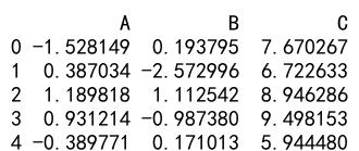
print(df.head())

Output:

Example 2: Calculating Pearson Correlation

import pandas as pd
import numpy as np

# Generating data
data = {'pandasdataframe.com_A': np.random.normal(0, 1, 100),
        'pandasdataframe.com_B': np.random.normal(1, 2, 100)}
df = pd.DataFrame(data)

# Calculating Pearson correlation
correlation_matrix = df.corr(method='pearson')
print(correlation_matrix)

Output:

Example 3: Calculating Spearman’s Rank Correlation

import pandas as pd
import numpy as np

# Generating data
data = {'pandasdataframe.com_A': np.random.rand(100),
        'pandasdataframe.com_B': np.random.rand(100)}
df = pd.DataFrame(data)

# Calculating Spearman's correlation
spearman_corr = df.corr(method='spearman')
print(spearman_corr)

Output:

Example 4: Calculating Kendall’s Tau Correlation

import pandas as pd
import numpy as np

# Generating data
data = {'pandasdataframe.com_A': np.random.rand(100),
        'pandasdataframe.com_B': np.random.rand(100)}
df = pd.DataFrame(data)

# Calculating Kendall's Tau correlation
kendall_corr = df.corr(method='kendall')
print(kendall_corr)

Output:

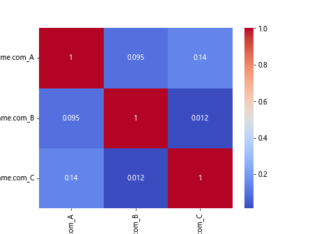
Example 5: Visualizing Correlation Matrix Using Seaborn

import pandas as pd
import numpy as np
import seaborn as sns
import matplotlib.pyplot as plt

# Generating data
data = {'pandasdataframe.com_A': np.random.normal(0, 1, 100),
        'pandasdataframe.com_B': np.random.normal(1, 2, 100),
        'pandasdataframe.com_C': np.random.normal(2, 3, 100)}
df = pd.DataFrame(data)

# Calculating Pearson correlation
correlation_matrix = df.corr()

# Plotting
sns.heatmap(correlation_matrix, annot=True, cmap='coolwarm')
plt.show()

Output:

Example 6: Handling Missing Data Before Correlation

import pandas as pd
import numpy as np

# Generating data with missing values
data = {'pandasdataframe.com_A': np.random.normal(0, 1, 100),
        'pandasdataframe.com_B': np.append(np.random.normal(1, 2, 95), [np.nan]*5)}
df = pd.DataFrame(data)

# Handling missing values
df.dropna(inplace=True)

# Calculating Pearson correlation
correlation_matrix = df.corr()
print(correlation_matrix)

Output:

Example 7: Correlation of a Subset of Columns

import pandas as pd
import numpy as np

# Generating data
data = {'pandasdataframe.com_A': np.random.normal(0, 1, 100),
        'pandasdataframe.com_B': np.random.normal(1, 2, 100),
        'pandasdataframe.com_C': np.random.uniform(5, 10, 100)}
df = pd.DataFrame(data)

# Calculating correlation for selected columns
selected_corr = df[['pandasdataframe.com_A', 'pandasdataframe.com_B']].corr()
print(selected_corr)

Output:

Example 8: Correlation Between Two Specific Columns

import pandas as pd
import numpy as np

# Generating data
data = {'pandasdataframe.com_A': np.random.normal(0, 1, 100),
        'pandasdataframe.com_B': np.random.normal(1, 2, 100)}
df = pd.DataFrame(data)

# Calculating Pearson correlation between two specific columns
correlation_value = df['pandasdataframe.com_A'].corr(df['pandasdataframe.com_B'])
print(correlation_value)

Output:

Example 9: Using Correlation for Feature Selection

import pandas as pd
import numpy as np

# Generating data
data = {'pandasdataframe.com_Feature1': np.random.normal(0, 1, 100),
        'pandasdataframe.com_Feature2': np.random.normal(1, 2, 100),
        'pandasdataframe.com_Target': np.random.randint(0, 2, 100)}
df = pd.DataFrame(data)

# Calculating correlation matrix
correlation_matrix = df.corr()

# Identifying highly correlated features
high_corr_features = correlation_matrix.index[abs(correlation_matrix["pandasdataframe.com_Target"]) > 0.5]
print(high_corr_features)

Output:

Example 10: Correlation Matrix with Non-Numeric Data

import pandas as pd
import numpy as np

# Generating data including categorical data
data = {'pandasdataframe.com_Category': ['A', 'B', 'A', 'C', 'B', 'A', 'C', 'B', 'A', 'C']*10,
        'pandasdataframe.com_Value': np.random.normal(0, 1, 100)}
df = pd.DataFrame(data)

# Converting categorical data to numeric
df['pandasdataframe.com_Category'] = df['pandasdataframe.com_Category'].astype('category').cat.codes

# Calculating Pearson correlation
correlation_matrix = df.corr()
print(correlation_matrix)

Output:

Pandas Correlation Conclusion

This article has provided a comprehensive guide to understanding and computing correlations in Pandas. By using the provided examples, you can start analyzing the relationships between variables in your own datasets. Remember, correlation does not imply causation, and further statistical testing may be necessary to draw meaningful conclusions from your data.