Pandas Cut

Pandas Cut

The pandas.cut function is a powerful tool for data transformation, particularly useful for dividing continuous values into discrete bins or categories. This is especially beneficial in data analysis and machine learning for feature engineering, enabling the transformation of numerical features into categorical ones. This comprehensive guide will delve into the pandas.cut function, exploring its syntax, parameters, and practical use cases. Additionally, we will provide detailed examples with complete, executable Pandas code snippets.

1. Introduction to pandas.cut

pandas.cut is used to segment and sort data values into bins or discrete intervals. This can be particularly useful for converting continuous variables into categorical ones, which can simplify analysis and model building. For example, transforming age into age groups or income into income brackets.

2. Syntax and Parameters

The pandas.cut function has a straightforward syntax:

pandas.cut(x, bins, right=True, labels=None, retbins=False, precision=3, include_lowest=False, duplicates='raise', ordered=True)

Parameters:

• x: Array-like input data to be binned.
• bins: Defines the bin edges. It can be an integer number of bins, an array of bin edges, or an IntervalIndex.
• right: Boolean indicating whether the bins include the rightmost edge or not.
• labels: Used to label the bins. If False, returns only integer indicators of bins.
• retbins: Whether to return the bins or not.
• precision: Precision at which to store and display the bin labels.
• include_lowest: Whether the first interval should include the lowest value.
• duplicates: Specifies how to handle duplicate bin edges.
• ordered: Whether the labels are ordered or not.

3. Basic Usage

Let’s start with a simple example of binning numerical data using pandas.cut.

Example 1: Basic Binning

import pandas as pd

# Sample data
data = pd.Series([1, 7, 5, 4, 6, 3, 8, 9, 2, 5])

# Binning the data
binned_data = pd.cut(data, bins=3)

print(binned_data)

Output:

In this example, we have a series of numerical data. The pd.cut function divides this data into three bins. The result is a categorical object indicating the bin each value belongs to.

4. Binning with Specified Intervals

We can specify exact bin edges to control the binning process more precisely.

Example 2: Specified Intervals

import pandas as pd

# Sample data
data = pd.Series([1, 7, 5, 4, 6, 3, 8, 9, 2, 5])

# Defining custom bin edges
bin_edges = [0, 2, 5, 7, 10]

# Binning the data with specified intervals
binned_data = pd.cut(data, bins=bin_edges)

print(binned_data)

Output:

Here, we define custom intervals for binning. The data points will be categorized based on these intervals.

5. Binning with Equal Frequency

Binning can also be done to ensure each bin has an equal number of data points. This is known as quantile-based binning.

Example 3: Equal Frequency Binning

import pandas as pd

# Sample data
data = pd.Series([1, 7, 5, 4, 6, 3, 8, 9, 2, 5])

# Binning into 4 bins with equal frequency
binned_data = pd.qcut(data, q=4)

print(binned_data)

Output:

In this example, pd.qcut is used to create bins such that each bin contains an equal number of data points.

6. Custom Labels for Bins

To make the binned data more interpretable, custom labels can be assigned to each bin.

Example 4: Custom Labels

import pandas as pd

# Sample data
data = pd.Series([1, 7, 5, 4, 6, 3, 8, 9, 2, 5])

# Custom bin labels
labels = ['Low', 'Medium', 'High']

# Binning the data with custom labels
binned_data = pd.cut(data, bins=3, labels=labels)

print(binned_data)

Output:

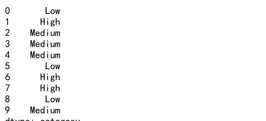
Here, we assign the labels ‘Low’, ‘Medium’, and ‘High’ to the three bins, making the binned data more meaningful.

7. Including Edge Cases

Sometimes, we want to include the lowest or highest values in our bins explicitly.

Example 5: Including Edge Cases

import pandas as pd

# Sample data
data = pd.Series([1, 7, 5, 4, 6, 3, 8, 9, 2, 5])

# Binning the data including the lowest value
binned_data = pd.cut(data, bins=3, include_lowest=True)

print(binned_data)

Output:

In this example, the lowest value is included in the first bin.

8. Working with DateTime Data

pandas.cut can also be used with datetime data, allowing for the binning of time series data into intervals.

Example 6: Binning DateTime Data

import pandas as pd

# Sample datetime data
data = pd.date_range(start='1/1/2020', periods=10, freq='D')

# Binning the datetime data
binned_data = pd.cut(data, bins=3)

print(binned_data)

Output:

This example demonstrates how to bin datetime data into three intervals.

9. Handling NaNs

pandas.cut can handle missing values (NaNs) gracefully, placing them in a separate bin if necessary.

Example 7: Handling NaNs

import pandas as pd
import numpy as np

# Sample data with NaN values
data = pd.Series([1, 7, 5, np.nan, 6, 3, 8, 9, np.nan, 5])

# Binning the data
binned_data = pd.cut(data, bins=3)

print(binned_data)

Output:

In this case, the NaN values are handled without causing errors, and they are excluded from the binning process.

10. Advanced Binning Techniques

More advanced techniques include combining pandas.cut with other functions for complex data transformations.

Example 8: Combining with GroupBy

import pandas as pd

# Sample data
df = pd.DataFrame({
    'value': [1, 7, 5, 4, 6, 3, 8, 9, 2, 5],
    'category': ['A', 'B', 'A', 'B', 'A', 'B', 'A', 'B', 'A', 'B']
})

# Binning the data within each group
df['binned'] = df.groupby('category')['value'].transform(lambda x: pd.cut(x, bins=3))

print(df)

Output:

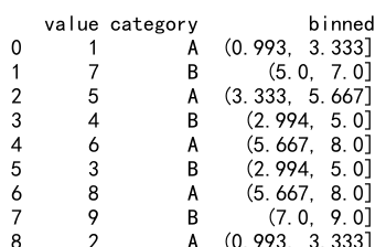
Here, we use pandas.cut in conjunction with groupby to bin data within each category separately.

11. Examples with Detailed Explanations

Let’s now dive into more detailed examples with explanations for each.

Example 9: Binning with Multiple Parameters

import pandas as pd

# Sample data
data = pd.Series([1, 7, 5, 4, 6, 3, 8, 9, 2, 5])

# Binning the data with custom parameters
binned_data = pd.cut(data, bins=4, right=False, labels=['Q1', 'Q2', 'Q3', 'Q4'], retbins=True, precision=1, include_lowest=True)

print(binned_data)

Output:

Explanation:

• bins=4: Specifies the number of bins.
• right=False: Indicates that the bins do not include the rightmost edge.
• labels=[‘Q1’, ‘Q2’, ‘Q3’, ‘Q4’]: Custom labels for each bin.
• retbins=True: Returns the bin edges along with the binned data.
• precision=1: Sets the precision for the bin labels.
• include_lowest=True: Ensures the lowest value is included in the first bin.

Example 10: Binning with IntervalIndex

import pandas as pd

# Sample data
data = pd.Series([1, 7, 5, 4, 6, 3, 8, 9, 2, 5])

# Creating an IntervalIndex
interval_index = pd.IntervalIndex.from_tuples([(0, 2), (2, 5), (5, 8), (8, 10)])

# Binning the data using IntervalIndex
binned_data = pd.cut(data, bins=interval_index)

print(binned_data)

Output:

Explanation:

• IntervalIndex: Defines custom intervals for binning.
• from_tuples: Creates the IntervalIndex from specified tuples.
• bins=interval_index: Uses the custom IntervalIndex for binning.

Example 11: Handling Duplicates

import pandas as pd

# Sample data
data = pd.Series([1, 7, 5, 4, 6, 3, 8, 9, 2, 5])

# Custom bin edges with duplicates
bin_edges = [0, 5, 5, 10]

# Binning the data with duplicate edges
try:
    binned_data = pd.cut(data, bins=bin_edges, duplicates='drop')
    print(binned_data)
except ValueError as e:
    print(f"Error: {e}")

Output:

Explanation:

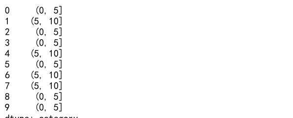
• duplicates=’drop’: Handles duplicate bin edges by dropping them.
• The try-except block ensures any errors due to duplicates are caught and printed.

Example 12: Binning with Large DataFrames

import pandas as pd
import numpy as np

# Generating large sample data
data = pd.DataFrame({
    'value': np.random.rand(10000) * 100,
    'category': np.random.choice(['A', 'B', 'C', 'D'], 10000)
})

# Binning the 'value' column
data['binned_value'] = pd.cut(data['value'], bins=10)

print(data.head())

Output:

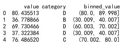
Explanation:

• np.random.rand(10000) * 100: Generates 10,000 random values between 0 and 100.
• np.random.choice: Randomly assigns one of four categories to each row.
• bins=10: Divides the ‘value’ column into 10 bins.

Example 13: Binning with Conditional Statements

import pandas as pd

# Sample data
data = pd.Series([1, 7, 5, 4, 6, 3, 8, 9, 2, 5])

# Defining a custom binning function
def custom_binning(x):
    if x < 3:
        return 'Low'
    elif x < 6:
        return 'Medium'
    else:
        return 'High'

# Applying the custom binning function
binned_data = data.apply(custom_binning)

print(binned_data)

Output:

Explanation:

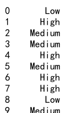
• custom_binning: Defines a function for custom binning logic.
• apply: Applies the custom binning function to each element in the series.

Example 14: Using Labels with Different Data Types

import pandas as pd

# Sample data
data = pd.Series([1, 7, 5, 4, 6, 3, 8, 9, 2, 5])

# Binning the data with different label types
binned_data = pd.cut(data, bins=3, labels=[1, 2, 3])

print(binned_data)

Output:

Explanation:

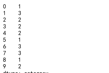
• labels=[1, 2, 3]: Assigns integer labels to each bin instead of the default string labels.

Example 15: Creating Custom Interval Labels

import pandas as pd

# Sample data
data = pd.Series([1, 7, 5, 4, 6, 3, 8, 9, 2, 5])

# Custom bin edges
bin_edges = [0, 3, 6, 9]

# Custom interval labels
labels = ['0-3', '3-6', '6-9']

# Binning the data with custom interval labels
binned_data = pd.cut(data, bins=bin_edges, labels=labels)

print(binned_data)

Output:

Explanation:

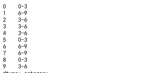
• labels=[‘0-3’, ‘3-6’, ‘6-9’]: Creates custom labels for the intervals based on the bin edges.

Example 16: Binning with Overlapping Bins

import pandas as pd

# Sample data
data = pd.Series([1, 7, 5, 4, 6, 3, 8, 9, 2, 5])

# Creating overlapping bins
bin_edges = [0, 5, 10, 15]

# Binning the data with overlapping bins
binned_data = pd.cut(data, bins=bin_edges, include_lowest=True, right=False)

print(binned_data)

Output:

Explanation:

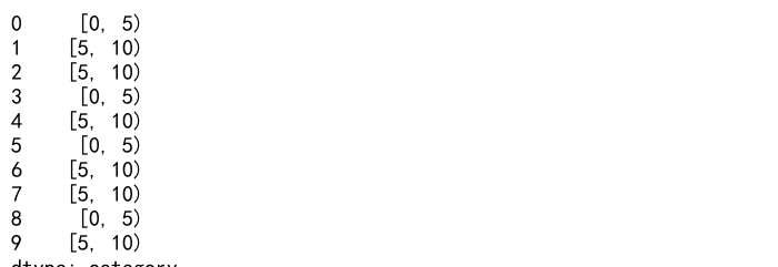
• right=False: Creates bins that do not include the rightmost edge, allowing for overlapping intervals.

Example 17: Binning with External Data

import pandas as pd

# External data for bin edges
bin_edges = pd.Series([0, 3, 6, 9])

# Sample data
data = pd.Series([1, 7, 5, 4, 6, 3, 8, 9, 2, 5])

# Binning the data using external bin edges
binned_data = pd.cut(data, bins=bin_edges, include_lowest=True)

print(binned_data)

Output:

Explanation:

• bin_edges: Uses a series of external data to define the bin edges.

Example 18: Binning with Dynamic Parameters

import pandas as pd
import numpy as np

# Dynamic bin count based on data range
data = pd.Series(np.random.rand(100) * 100)
bin_count = int(data.max() / 10)

# Binning the data dynamically
binned_data = pd.cut(data, bins=bin_count)

print(binned_data)

Output:

Explanation:

• bin_count: Dynamically calculates the number of bins based on the data range.
• np.random.rand(100) * 100: Generates 100 random values between 0 and 100.

Pandas Cut Conclusion

The pandas.cut function is an essential tool for data scientists and analysts, allowing for the transformation of continuous data into categorical data, which can be crucial for various analytical and machine learning tasks. This guide covered the fundamental aspects and advanced techniques of using pandas.cut, providing a range of examples to illustrate its versatility and power. By mastering pandas.cut, you can enhance your data preprocessing and feature engineering workflows, enabling more effective data analysis and modeling.

Remember, the key to effectively using pandas.cut lies in understanding your data and the specific requirements of your analysis. With practice, you will become proficient in applying this powerful function to a wide variety of datasets and analytical scenarios.