Pandas Create DataFrame from Another DataFrame

Pandas Create DataFrame from Another DataFrame

Pandas is an essential library for data analysis in Python, and one of its powerful features is the ability to create a new DataFrame from an existing one. This functionality is crucial for data cleaning, transformation, and manipulation tasks. In this article, we will explore various methods to create DataFrames from other DataFrames, providing detailed explanations and practical examples.

1. Introduction

Creating a DataFrame from another DataFrame is a common task in data analysis workflows. This article will cover various methods to achieve this using the pandas library, with detailed code examples and explanations for each method.

2. Copying DataFrames

Creating a copy of an existing DataFrame is often the first step when you want to manipulate data without altering the original DataFrame.

import pandas as pd

# Create original DataFrame
df_original = pd.DataFrame({
    'A': [1, 2, 3],
    'B': ['x', 'y', 'z']
})

# Create a copy of the DataFrame
df_copy = df_original.copy()

print(df_copy)

Output:

Explanation:
– The copy method creates a deep copy of the original DataFrame df_original.
– This ensures that changes to df_copy do not affect df_original.

3. Selecting Specific Columns

You can create a new DataFrame by selecting specific columns from an existing DataFrame.

import pandas as pd

# Create original DataFrame
df_original = pd.DataFrame({
    'A': [1, 2, 3],
    'B': ['x', 'y', 'z'],
    'C': [4, 5, 6]
})

# Select specific columns to create a new DataFrame
df_selected_columns = df_original[['A', 'C']]

print(df_selected_columns)

Output:

Explanation:
– The new DataFrame df_selected_columns is created by selecting columns ‘A’ and ‘C’ from df_original.
– This is useful when you need only a subset of columns for analysis.

4. Filtering Rows

Creating a DataFrame by filtering rows based on conditions is a common task.

import pandas as pd

# Create original DataFrame
df_original = pd.DataFrame({
    'A': [1, 2, 3, 4],
    'B': ['x', 'y', 'z', 'w']
})

# Filter rows where column 'A' is greater than 2
df_filtered_rows = df_original[df_original['A'] > 2]

print(df_filtered_rows)

Output:

Explanation:
– The new DataFrame df_filtered_rows contains rows where the values in column ‘A’ are greater than 2.
– This is useful for filtering data based on specific conditions.

5. Adding Calculated Columns

You can create a new DataFrame by adding calculated columns to an existing DataFrame.

import pandas as pd

# Create original DataFrame
df_original = pd.DataFrame({
    'A': [1, 2, 3],
    'B': [4, 5, 6]
})

# Add a new calculated column 'C' as the sum of 'A' and 'B'
df_with_calculated_column = df_original.copy()
df_with_calculated_column['C'] = df_with_calculated_column['A'] + df_with_calculated_column['B']

print(df_with_calculated_column)

Output:

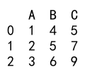
Explanation:
– A new column ‘C’ is added to df_with_calculated_column, which is the sum of columns ‘A’ and ‘B’.
– Adding calculated columns is useful for creating derived metrics.

6. Using Conditions to Modify DataFrames

Creating a DataFrame by modifying an existing one based on conditions is often required.

import pandas as pd

# Create original DataFrame
df_original = pd.DataFrame({
    'A': [1, 2, 3, 4],
    'B': [4, 5, 6, 7]
})

# Create a new DataFrame with a condition
df_condition = df_original.copy()
df_condition['C'] = df_condition['A'].apply(lambda x: 'High' if x > 2 else 'Low')

print(df_condition)

Output:

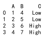
Explanation:
– A new column ‘C’ is added to df_condition, where the value is ‘High’ if the corresponding value in ‘A’ is greater than 2, otherwise ‘Low’.
– This technique is useful for categorizing data based on conditions.

7. Merging and Joining DataFrames

Merging and joining are powerful ways to create a new DataFrame from two or more DataFrames.

import pandas as pd

# Create two DataFrames
df1 = pd.DataFrame({
    'key': ['A', 'B', 'C'],
    'value1': [1, 2, 3]
})

df2 = pd.DataFrame({
    'key': ['A', 'B', 'D'],
    'value2': [4, 5, 6]
})

# Merge the DataFrames on the 'key' column
df_merged = pd.merge(df1, df2, on='key', how='inner')

print(df_merged)

Output:

Explanation:
– The merge function is used to combine df1 and df2 on the ‘key’ column, performing an inner join.
– This method is essential for combining data from different sources based on a common key.

8. Grouping and Aggregating Data

Creating a DataFrame by grouping and aggregating data is a powerful technique for summarizing data.

import pandas as pd

# Create original DataFrame
df_original = pd.DataFrame({
    'Category': ['A', 'A', 'B', 'B'],
    'Value': [10, 20, 30, 40]
})

# Group by 'Category' and calculate the mean of 'Value'
df_grouped = df_original.groupby('Category').agg({'Value': 'mean'}).reset_index()

print(df_grouped)

Output:

Explanation:
– The data is grouped by the ‘Category’ column, and the mean of the ‘Value’ column is calculated.
– Grouping and aggregating are useful for summarizing data and extracting meaningful insights.

9. Pivoting DataFrames

Pivoting is used to reshape data for better analysis and visualization.

import pandas as pd

# Create original DataFrame
df_original = pd.DataFrame({
    'Date': ['2021-01', '2021-02', '2021-01', '2021-02'],
    'Category': ['A', 'A', 'B', 'B'],
    'Value': [10, 15, 20, 25]
})

# Pivot the DataFrame
df_pivot = df_original.pivot(index='Date', columns='Category', values='Value')

print(df_pivot)

Output:

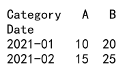
Explanation:
– The pivot function reshapes the DataFrame, setting ‘Date’ as the index, ‘Category’ as columns, and ‘Value’ as the values.
– Pivoting is useful for transforming data for easier analysis.

10. Using Apply and Lambda Functions

The apply method combined with lambda functions allows for flexible row and column transformations.

import pandas as pd

# Create original DataFrame
df_original = pd.DataFrame({
    'A': [1, 2, 3],
    'B': [4, 5, 6]
})

# Apply a lambda function to create a new column
df_apply = df_original.copy()
df_apply['C'] = df_apply.apply(lambda row: row['A'] * row['B'], axis=1)

print(df_apply)

Output:

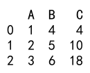
Explanation:
– The apply method applies a lambda function to each row, creating a new column ‘C’ as the product of ‘A’ and ‘B’.
– This method is useful for complex transformations that require custom logic.

11. Handling Missing Data

Creating a DataFrame by handling missing data is crucial for data quality.

import pandas as pd

# Create original DataFrame with missing values
df_original = pd.DataFrame({
    'A': [1, 2, None],
    'B': [None, 2, 3]
})

# Fill missing values with a specified value
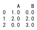
df_filled = df_original.fillna(0)

print(df_filled)

Output:

Explanation:
– The fillna method replaces missing values with 0.
– Handling missing data is essential to ensure accurate analysis.

12. Sorting DataFrames

Sorting DataFrames helps in organizing data in a specific order.

import pandas as pd

# Create original DataFrame
df_original = pd.DataFrame({
    'A': [3, 1, 2],
    'B': ['x', 'y', 'z']
})

# Sort the DataFrame by column 'A'
df_sorted = df_original.sort_values(by='A')

print(df_sorted)

Output:

Explanation:
– The sort_values method sorts the DataFrame by column ‘A’ in ascending order.
– Sorting is useful for organizing data for better readability and analysis.

13. Sampling Data

Sampling is useful for creating a smaller subset of data for analysis or testing.

import pandas as pd

# Create original DataFrame
df_original = pd.DataFrame({
    'A': range(1, 101),
    'B': ['x'] * 100
})

# Sample 10 rows from the DataFrame
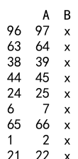
df_sampled = df_original.sample(n=10)

print(df_sampled)

Output:

Explanation:
– The sample method randomly selects 10 rows from the original DataFrame.
– Sampling is helpful when dealing with large datasets and you need a smaller sample for quick analysis.

14. Reindexing and Renaming

Reindexing and renaming DataFrames are common operations for aligning data.

import pandas as pd

# Create original DataFrame
df_original = pd.DataFrame({
    'A': [1, 2, 3],
    'B': ['x', 'y', 'z']
}, index=['one', 'two', 'three'])

# Reindex the DataFrame
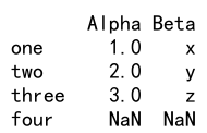
df_reindexed = df_original.reindex(['one', 'two', 'three', 'four'])

# Rename columns
df_renamed = df_reindexed.rename(columns={'A': 'Alpha', 'B': 'Beta'})

print(df_renamed)

Output:

Explanation:
– The reindex method reindexes the DataFrame to include a new index ‘four’.
– The rename method renames columns ‘A’ to ‘Alpha’ and ‘B’ to ‘Beta’.
– These methods are useful for aligning and renaming data for consistency.

15. Concatenating DataFrames

Concatenating DataFrames allows for combining multiple DataFrames into one.

import pandas as pd

# Create two DataFrames
df1 = pd.DataFrame({
    'A': [1, 2],
    'B': ['x', 'y']
})

df2 = pd.DataFrame({
    'A': [3, 4],
    'B': ['z', 'w']
})

# Concatenate the DataFrames
df_concatenated = pd.concat([df1, df2], ignore_index=True)

print(df_concatenated)

Output:

Explanation:
– The concat function combines df1 and df2 into a single DataFrame, resetting the index.
– Concatenating is useful for appending data from different sources.

16. Using Query for Filtering

The query method provides a powerful way to filter data based on conditions.

import pandas as pd

# Create original DataFrame
df_original = pd.DataFrame({
    'A': [1, 2, 3, 4],
    'B': ['x', 'y', 'z', 'w']
})

# Filter rows using query
df_query = df_original.query('A > 2')

print(df_query)

Output:

Explanation:
– The query method filters rows where the value in column ‘A’ is greater than 2.
– This method is useful for filtering data using a query-like syntax.

17. Transposing DataFrames

Transposing switches the rows and columns of a DataFrame.

import pandas as pd

# Create original DataFrame
df_original = pd.DataFrame({
    'A': [1, 2, 3],
    'B': ['x', 'y', 'z']
})

# Transpose the DataFrame
df_transposed = df_original.T

print(df_transposed)

Output:

Explanation:
– The T attribute transposes the DataFrame, swapping rows and columns.
– Transposing is useful for reorienting data for analysis or visualization.

18. Exploding Lists into Rows

Exploding lists within DataFrame cells into separate rows is useful for normalizing data.

import pandas as pd

# Create original DataFrame
df_original = pd.DataFrame({
    'A': [1, 2],
    'B': [['x', 'y'], ['z', 'w']]
})

# Explode lists into rows
df_exploded = df_original.explode('B')

print(df_exploded)

Output:

Explanation:
– The explode method transforms lists in column ‘B’ into separate rows.
– This method is useful for normalizing data stored in list-like structures.

19. Stacking and Unstacking DataFrames

Stacking and unstacking reshape DataFrames for hierarchical indexing and pivoting.

import pandas as pd

# Create original DataFrame
df_original = pd.DataFrame({
    'A': [1, 2],
    'B': [3, 4]
}, index=['x', 'y'])

# Stack the DataFrame
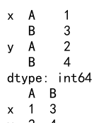
df_stacked = df_original.stack()

# Unstack the DataFrame
df_unstacked = df_stacked.unstack()

print(df_stacked)
print(df_unstacked)

Output:

Explanation:
– The stack method pivots columns into rows, creating a Series with a multi-level index.
– The unstack method reverses this operation, pivoting the rows back into columns.
– These methods are useful for hierarchical data manipulation.

20. Pandas Create DataFrame from Another DataFrame Conclusion

Creating DataFrames from existing DataFrames using pandas is a fundamental aspect of data manipulation. This article has covered various methods to achieve this, including copying, selecting, filtering, adding columns, merging, grouping, pivoting, and more. Each method is accompanied by practical examples to demonstrate its usage.