Pandas Cut Histogram

Pandas Cut Histogram

Pandas is a powerful library in Python for data manipulation and analysis. One of the key functionalities it offers is the ability to create histograms, particularly by using the cut function. This article will delve deeply into the pandas.cut function, exploring its usage, providing detailed examples, and explaining the outputs. By the end of this article, you should have a thorough understanding of how to use pandas.cut to create histograms and how to interpret the results.

Pandas Cut Histogram Table of Contents

1. Introduction to pandas.cut
2. Understanding Binning
3. Creating Simple Bins with pandas.cut
4. Advanced Binning Techniques
5. Visualizing Binned Data
6. Case Studies
7. Common Pitfalls and How to Avoid Them
8. Conclusion

1. Introduction to pandas.cut

The pandas.cut function is used to segment and sort data values into bins or categories. This is particularly useful in data analysis for discretizing continuous variables into categorical ones, enabling the creation of histograms and frequency tables.

What is pandas.cut?

The pandas.cut function divides the data into discrete intervals, or bins. It’s primarily used for converting continuous numerical data into categorical data. The function returns an array of intervals which are helpful for statistical analysis and plotting.

Syntax

pandas.cut(x, bins, right=True, labels=None, retbins=False, precision=3, include_lowest=False, duplicates='raise')

• x: The input array to be binned.
• bins: The criteria to bin by. Can be an integer (for equal-width bins) or a sequence of scalars (for custom bins).
• right: Indicates whether bins include the rightmost edge or not.
• labels: Used as labels for the resulting bins. Must be the same length as the resulting bins.
• retbins: Whether to return the bins or not.
• precision: Precision at which to store and display the bins labels.
• include_lowest: Whether the first interval should be left-inclusive or not.
• duplicates: How to handle bin edges that are not unique.

Why Use pandas.cut?

pandas.cut is useful for:
– Histogram creation: Segmenting data into intervals to visualize frequency distributions.
– Data discretization: Converting continuous data into categorical data.
– Statistical analysis: Grouping data for statistical summaries.

2. Understanding Binning

Binning is the process of transforming continuous data into discrete bins. This helps in reducing the effect of minor observation errors and can make the data easier to understand and visualize.

Types of Binning

1. Equal-Width Binning: Each bin has the same width or range.
2. Equal-Frequency Binning: Each bin has the same number of observations.
3. Custom Binning: Bins are defined by custom boundaries.

Examples

Example 1: Equal-Width Binning

import pandas as pd
import numpy as np

data = np.random.rand(100)
bins = pd.cut(data, 5)
print(bins)

Output:

Explanation: This code generates 100 random numbers between 0 and 1 and bins them into 5 equal-width bins.

Example 2: Custom Binning

import pandas as pd
import numpy as np

data = np.random.rand(100)
bins = pd.cut(data, [0, 0.2, 0.4, 0.6, 0.8, 1.0])
print(bins)

Output:

Explanation: Here, we define custom bins for the same data set, specifying the exact boundaries of each bin.

3. Creating Simple Bins with pandas.cut

Creating bins is straightforward with pandas.cut. This section will cover basic usage.

Basic Usage

Example 3: Simple Binning with Labels

import pandas as pd
import numpy as np

data = np.random.rand(100)
bins = pd.cut(data, bins=5, labels=["Very Low", "Low", "Medium", "High", "Very High"])
print(bins)

Output:

Explanation: This example bins the data into 5 intervals and labels them from “Very Low” to “Very High”.

Example 4: Returning Bin Edges

import pandas as pd
import numpy as np

data = np.random.rand(100)
bins, bin_edges = pd.cut(data, bins=5, retbins=True)
print(bins)
print(bin_edges)

Output:

Explanation: This example returns both the binned data and the edges of the bins.

4. Advanced Binning Techniques

Advanced binning allows for more control over how data is segmented.

Binning with qcut

pandas.qcut bins data into quantiles, ensuring each bin has approximately the same number of observations.

Example 5: Equal-Frequency Binning with qcut

import pandas as pd
import numpy as np

data = np.random.rand(100)
bins = pd.qcut(data, 4, labels=["Q1", "Q2", "Q3", "Q4"])
print(bins)

Output:

Explanation: This example bins the data into four quantiles and labels them from Q1 to Q4.

Custom Binning with Duplicates Handling

Example 6: Handling Duplicate Bin Edges

import pandas as pd
import numpy as np

data = np.random.rand(100)
bins = pd.cut(data, bins=[0, 0.3, 0.3, 0.6, 1.0], duplicates='drop')
print(bins)

Output:

Explanation: Here, duplicate bin edges are handled by dropping them.

Including Lowest Value

Example 7: Including the Lowest Value

import pandas as pd
import numpy as np

data = np.random.rand(100)
bins = pd.cut(data, bins=5, include_lowest=True)
print(bins)

Output:

Explanation: This ensures that the lowest value in the data is included in the first bin.

5. Visualizing Binned Data

Visualization helps in understanding the distribution of the data across bins.

Plotting Histograms

Example 8: Simple Histogram Plot

import pandas as pd
import numpy as np
import matplotlib.pyplot as plt

data = np.random.rand(100)
bins = pd.cut(data, bins=5)
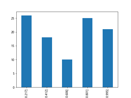
bins.value_counts().plot(kind='bar')
plt.show()

Output:

Explanation: This example bins the data and plots a histogram of the bin counts using Matplotlib.

Adding Custom Labels

Example 9: Histogram with Custom Labels

import pandas as pd
import numpy as np
import matplotlib.pyplot as plt

data = np.random.rand(100)
bins = pd.cut(data, bins=5, labels=["Very Low", "Low", "Medium", "High", "Very High"])
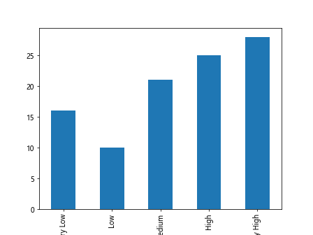
bins.value_counts().plot(kind='bar')
plt.show()

Output:

Explanation: This example is similar to the previous one but includes custom labels for each bin.

6. Case Studies

Case studies provide practical applications of pandas.cut.

Case Study 1: Income Brackets

Example 10: Income Bracket Binning

import pandas as pd

income_data = [20000, 35000, 50000, 75000, 120000, 150000, 200000]
bins = [0, 30000, 60000, 100000, 150000, 200000]
labels = ["Low", "Lower-Middle", "Middle", "Upper-Middle", "High"]
income_bins = pd.cut(income_data, bins, labels=labels)
print(income_bins)

Output:

Explanation: This example bins income data into predefined brackets and labels them accordingly.

Case Study 2: Age Grouping

Example 11: Grouping Ages into Categories

import pandas as pd

age_data = [5, 12, 17, 19, 24, 35, 45, 60, 75, 85]
bins = [0, 12, 18, 35, 50, 100]
labels = ["Child", "Teen", "Young Adult", "Adult", "Senior"]
age_bins = pd.cut(age_data, bins, labels=labels)
print(age_bins)

Output:

Explanation: This example categorizes ages into various life stages.

Case Study 3: Sales Performance

Example 12: Categorizing Sales Performance

import pandas as pd

sales_data = [100, 150, 200, 250, 300, 350, 400, 450, 500]
bins = [0, 200, 300, 400, 500]
labels = ["Poor", "Average", "Good", "Excellent"]
sales_bins = pd.cut(sales_data, bins, labels=labels)
print(sales_bins)

Output:

Explanation: This example bins sales data into performance categories.

7. Common Pitfalls and How to Avoid Them

While using pandas.cut, several common pitfalls may arise.

Handling NaN Values

Example 13: Binning with NaN Values

import pandas as pd
import numpy as np

data = [1, 2, 3, 4, np.nan, 6, 7, 8, 9, 10]
bins = pd.cut(data, bins=3)
print(bins)

Output:

Explanation: This example demonstrates how pandas.cut handles NaN values by default.

Duplicate Bin Edges

Example 14: Avoiding Duplicate Edges

import pandas as pd
import numpy as np

data = np.random.rand(100)
try:
    bins = pd.cut(data, bins=[0, 0.5, 0.5, 1.0])
except ValueError as e:
    print(f"Error: {e}")

Output:

Explanation: This example shows an error raised due to duplicate bin edges.

Precision Issues

Example 15: Setting Precision

import pandas as pd
import numpy as np

data = np.random.rand(100)
bins = pd.cut(data, bins=5, precision=2)
print(bins)

Output:

Explanation: This example sets the precision of the bin edges to 2 decimal places.

8. Pandas Cut Histogram Conclusion

The pandas.cut function is a versatile tool for data binning, allowing for the transformation of continuous data into discrete intervals. This is crucial for statistical analysis and data visualization. By understanding and utilizing pandas.cut, you can gain deeper insights into your data and present it more effectively.