Pandas Filter-Pandas Dataframe

Pandas Filter

Pandas is a powerful data manipulation library in Python that provides efficient and flexible tools for working with structured data. One of the most fundamental operations in data analysis is filtering, which allows you to select specific rows or columns from a DataFrame based on certain conditions. In this comprehensive guide, we’ll explore various techniques and methods for filtering data in pandas, covering simple and complex filtering operations, along with numerous examples and explanations.

1. Introduction to Pandas Filtering

Filtering in pandas refers to the process of selecting a subset of data from a DataFrame or Series based on specified conditions. This operation is crucial for data analysis, as it allows you to focus on specific portions of your dataset that meet certain criteria. Pandas provides several methods for filtering, including boolean indexing, the loc and iloc accessors, and the query() method.

Let’s start with a basic example to illustrate the concept of filtering:

import pandas as pd

# Create a sample DataFrame
df = pd.DataFrame({
    'Name': ['John', 'Emma', 'Alex', 'Sarah', 'Michael'],
    'Age': [28, 32, 25, 30, 35],
    'City': ['New York', 'London', 'Paris', 'Tokyo', 'Sydney'],
    'Salary': [50000, 60000, 45000, 55000, 65000]
})

# Filter rows where Age is greater than 30
filtered_df = df[df['Age'] > 30]

print("Original DataFrame:")
print(df)
print("\nFiltered DataFrame:")
print(filtered_df)

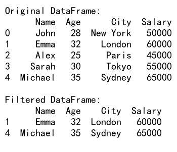
Output:

Pandas Filter

In this example, we create a simple DataFrame with information about employees. We then filter the DataFrame to select only the rows where the ‘Age’ is greater than 30. The resulting filtered_df contains only the rows that meet this condition.

2. Boolean Indexing

Boolean indexing is one of the most common and versatile methods for filtering data in pandas. It involves creating a boolean mask (a Series of True/False values) based on a condition and using this mask to select rows from the DataFrame.

2.1 Simple Boolean Indexing

Let’s look at a more detailed example of boolean indexing:

import pandas as pd

# Create a sample DataFrame
df = pd.DataFrame({
    'Product': ['Laptop', 'Smartphone', 'Tablet', 'Smartwatch', 'Headphones'],
    'Price': [1200, 800, 500, 300, 150],
    'Stock': [50, 100, 75, 200, 300],
    'Category': ['Electronics', 'Electronics', 'Electronics', 'Wearables', 'Audio']
})

# Filter products with price greater than 500
expensive_products = df[df['Price'] > 500]

# Filter products with stock less than 100
low_stock_products = df[df['Stock'] < 100]

print("All products:")
print(df)
print("\nExpensive products:")
print(expensive_products)
print("\nLow stock products:")
print(low_stock_products)

Output:

Pandas Filter

In this example, we create a DataFrame of products and demonstrate two filtering operations:
1. Selecting products with a price greater than 500
2. Selecting products with stock less than 100

The boolean condition (e.g., df['Price'] > 500) creates a Series of True/False values, which is then used to index the DataFrame.

2.2 Combining Multiple Conditions

You can combine multiple conditions using logical operators like & (and), | (or), and ~ (not). When combining conditions, it’s important to use parentheses to ensure correct precedence.

import pandas as pd

# Create a sample DataFrame
df = pd.DataFrame({
    'Name': ['Alice', 'Bob', 'Charlie', 'David', 'Eve'],
    'Age': [25, 30, 35, 28, 32],
    'Department': ['Sales', 'IT', 'HR', 'Marketing', 'Finance'],
    'Salary': [50000, 60000, 55000, 52000, 58000]
})

# Filter employees in IT or Finance departments with salary > 55000
filtered_df = df[(df['Department'].isin(['IT', 'Finance'])) & (df['Salary'] > 55000)]

print("Original DataFrame:")
print(df)
print("\nFiltered DataFrame:")
print(filtered_df)

Output:

Pandas Filter

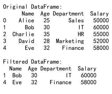
In this example, we combine two conditions:
1. The employee’s department is either IT or Finance (using the isin() method)
2. The employee’s salary is greater than 55000

The & operator is used to combine these conditions, and parentheses are used to ensure correct evaluation.

3. Using `loc` and `iloc` for Filtering

The loc and iloc accessors provide a powerful way to select data based on labels or integer positions. While they are primarily used for data selection, they can also be employed for filtering operations.

3.1 Filtering with `loc`

The loc accessor is label-based and can be used with boolean arrays for filtering:

import pandas as pd

# Create a sample DataFrame
df = pd.DataFrame({
    'Date': pd.date_range(start='2023-01-01', periods=10),
    'Value': [10, 15, 8, 12, 20, 18, 22, 25, 19, 30],
    'Category': ['A', 'B', 'A', 'C', 'B', 'A', 'C', 'B', 'A', 'C']
})

# Filter rows where Value is greater than 15 and Category is either 'A' or 'B'
filtered_df = df.loc[(df['Value'] > 15) & (df['Category'].isin(['A', 'B']))]

print("Original DataFrame:")
print(df)
print("\nFiltered DataFrame:")
print(filtered_df)

Output:

Pandas Filter

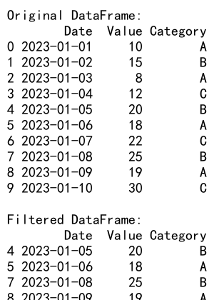
In this example, we use loc to filter the DataFrame based on two conditions:
1. The ‘Value’ column is greater than 15
2. The ‘Category’ column is either ‘A’ or ‘B’

The loc accessor allows us to combine these conditions and select the rows that meet both criteria.

3.2 Filtering with `iloc`

The iloc accessor is integer-based and can be used to filter rows based on their positions:

import pandas as pd

# Create a sample DataFrame
df = pd.DataFrame({
    'Product': ['Laptop', 'Smartphone', 'Tablet', 'Smartwatch', 'Headphones'],
    'Price': [1200, 800, 500, 300, 150],
    'Stock': [50, 100, 75, 200, 300],
    'Category': ['Electronics', 'Electronics', 'Electronics', 'Wearables', 'Audio']
})

# Filter every other row
filtered_df = df.iloc[::2]

print("Original DataFrame:")
print(df)
print("\nFiltered DataFrame (every other row):")
print(filtered_df)

Output:

Pandas Filter

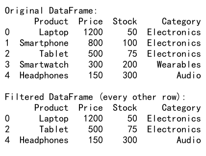
In this example, we use iloc to select every other row from the DataFrame. The slice ::2 means “start at the beginning, go to the end, with a step of 2”.

4. Using the `query()` Method

The query() method provides a concise way to filter DataFrames using a string expression. It can be more readable for complex filtering conditions and potentially more efficient for large DataFrames.

import pandas as pd

# Create a sample DataFrame
df = pd.DataFrame({
    'Name': ['John', 'Emma', 'Alex', 'Sarah', 'Michael'],
    'Age': [28, 32, 25, 30, 35],
    'City': ['New York', 'London', 'Paris', 'Tokyo', 'Sydney'],
    'Salary': [50000, 60000, 45000, 55000, 65000]
})

# Filter using query method
filtered_df = df.query('Age > 30 and City != "New York"')

print("Original DataFrame:")
print(df)
print("\nFiltered DataFrame:")
print(filtered_df)

Output:

Pandas Filter

In this example, we use the query() method to filter the DataFrame. The query string 'Age > 30 and City != "New York"' selects rows where the age is greater than 30 and the city is not New York.

5. Filtering with String Methods

Pandas provides string methods that can be applied to string columns for filtering based on text patterns.

import pandas as pd

# Create a sample DataFrame
df = pd.DataFrame({
    'Name': ['John Smith', 'Emma Johnson', 'Alex Brown', 'Sarah Davis', 'Michael Wilson'],
    'Email': ['[email protected]', '[email protected]', '[email protected]', '[email protected]', '[email protected]'],
    'Department': ['Sales', 'Marketing', 'IT', 'HR', 'Finance']
})

# Filter rows where the email contains 'pandasdataframe.com'
filtered_df = df[df['Email'].str.contains('pandasdataframe.com')]

print("Original DataFrame:")
print(df)
print("\nFiltered DataFrame:")
print(filtered_df)

Output:

Pandas Filter

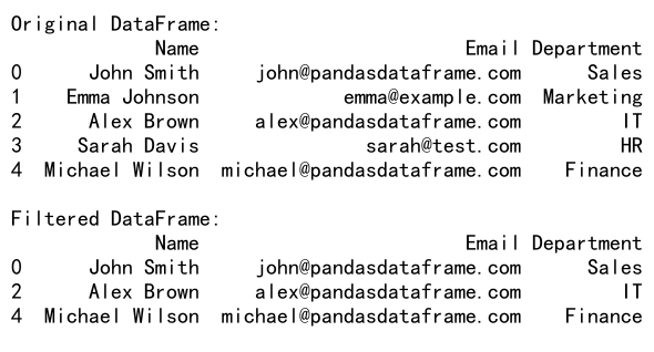
In this example, we use the str.contains() method to filter rows where the email address contains ‘pandasdataframe.com’. This is useful for filtering based on partial string matches.

6. Filtering with Regular Expressions

Regular expressions provide a powerful way to filter data based on complex string patterns. Pandas integrates well with regular expressions through its string methods.

import pandas as pd

# Create a sample DataFrame
df = pd.DataFrame({
    'Name': ['John Smith', 'Emma Johnson', 'Alex Brown', 'Sarah Davis', 'Michael Wilson'],
    'Phone': ['123-456-7890', '987-654-3210', '456-789-0123', '789-012-3456', '321-654-9870'],
    'Email': ['[email protected]', '[email protected]', '[email protected]', '[email protected]', '[email protected]']
})

# Filter rows where the phone number starts with '123' or '456'
filtered_df = df[df['Phone'].str.match(r'^(123|456)')]

print("Original DataFrame:")
print(df)
print("\nFiltered DataFrame:")
print(filtered_df)

Output:

Pandas Filter

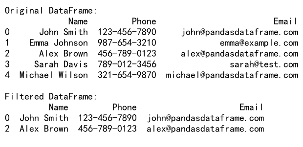
In this example, we use a regular expression with the str.match() method to filter rows where the phone number starts with either ‘123’ or ‘456’. The regular expression ^(123|456) matches strings that start (^) with either 123 or 456.

7. Filtering Date and Time Data

Pandas provides powerful capabilities for working with date and time data, including filtering based on date ranges or specific time conditions.

import pandas as pd

# Create a sample DataFrame with date and time data
df = pd.DataFrame({
    'Date': pd.date_range(start='2023-01-01', end='2023-12-31', freq='D'),
    'Value': range(365)
})

# Filter rows for the month of March
march_data = df[(df['Date'].dt.month == 3)]

# Filter rows for weekends
weekend_data = df[df['Date'].dt.dayofweek.isin([5, 6])]

print("Original DataFrame (first 5 rows):")
print(df.head())
print("\nMarch data:")
print(march_data)
print("\nWeekend data (first 5 rows):")
print(weekend_data.head())

Output:

Pandas Filter

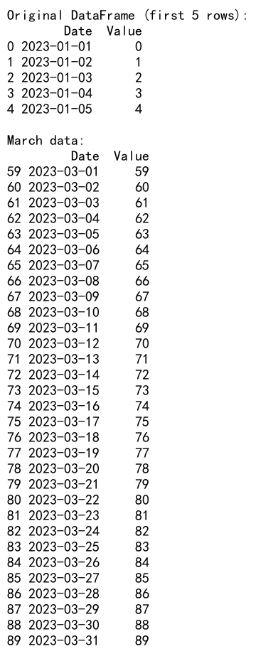
In this example, we demonstrate two types of date-based filtering:
1. Selecting all rows for the month of March using the dt.month accessor
2. Selecting all weekend days (Saturday and Sunday) using the dt.dayofweek accessor

These methods allow for powerful and flexible filtering of time series data.

8. Filtering with `isin()` Method

The isin() method is useful when you want to filter rows based on whether a column’s values are in a specified list.

import pandas as pd

# Create a sample DataFrame
df = pd.DataFrame({
    'Name': ['John', 'Emma', 'Alex', 'Sarah', 'Michael'],
    'Department': ['Sales', 'Marketing', 'IT', 'HR', 'Finance'],
    'Project': ['Alpha', 'Beta', 'Gamma', 'Delta', 'Epsilon']
})

# List of departments to filter
target_departments = ['Sales', 'IT', 'Finance']

# Filter rows where Department is in the target list
filtered_df = df[df['Department'].isin(target_departments)]

print("Original DataFrame:")
print(df)
print("\nFiltered DataFrame:")
print(filtered_df)

Output:

Pandas Filter

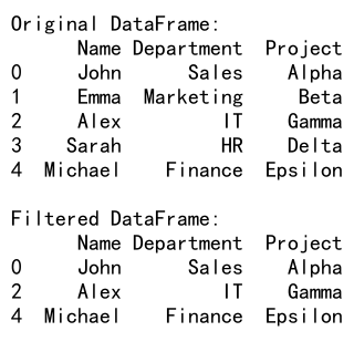
In this example, we use the isin() method to filter rows where the ‘Department’ is one of the values in the target_departments list. This is particularly useful when you have a predefined set of values you want to match against.

9. Filtering with `between()` Method

The between() method is a convenient way to filter values within a specific range, inclusive of the endpoints.

import pandas as pd

# Create a sample DataFrame
df = pd.DataFrame({
    'Product': ['A', 'B', 'C', 'D', 'E', 'F', 'G', 'H', 'I', 'J'],
    'Price': [10, 25, 30, 45, 50, 65, 70, 85, 90, 100]
})

# Filter products with prices between 30 and 70 (inclusive)
filtered_df = df[df['Price'].between(30, 70)]

print("Original DataFrame:")
print(df)
print("\nFiltered DataFrame:")
print(filtered_df)

Output:

Pandas Filter

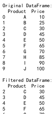
In this example, we use the between() method to filter rows where the ‘Price’ is between 30 and 70, inclusive. This is equivalent to df[(df['Price'] >= 30) & (df['Price'] <= 70)], but it’s more concise and readable.

10. Filtering with Custom Functions

You can use custom functions with apply() to create complex filtering conditions that aren’t easily expressed with standard comparison operators.

import pandas as pd

# Create a sample DataFrame
df = pd.DataFrame({
    'Name': ['John', 'Emma', 'Alex', 'Sarah', 'Michael'],
    'Score1': [85, 92, 78, 95, 88],
    'Score2': [90, 88, 82, 93, 85]
})

# Custom function to calculate average score
def high_average(row):
    return (row['Score1'] + row['Score2']) / 2 > 90

# Apply the custom function to filter rows
filtered_df = df[df.apply(high_average, axis=1)]

print("Original DataFrame:")
print(df)
print("\nFiltered DataFrame:")
print(filtered_df)

Output:

Pandas Filter

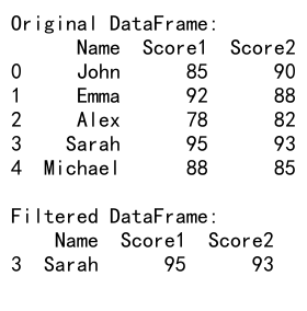
In this example, we define a custom function high_average that calculates the average of two scores and returns True if the average is greater than 90. We then use apply() with this function to filter the DataFrame, selecting only the rows where the average score is above 90.

11. Filtering with `nsmallest()` and `nlargest()`

The nsmallest() and nlargest() methods are useful for selecting a specific number of rows based on the values in a particular column.

import pandas as pd

# Create a sample DataFrame
df = pd.DataFrame({
    'Name': ['John', 'Emma', 'Alex', 'Sarah', 'Michael', 'Olivia', 'Daniel'],
    'Age': [28, 32, 25, 30, 35, 27, 33],
    'Salary': [50000, 60000, 45000, 55000, 65000, 52000, 58000]
})

# Select the 3 employees with the highest salaries
top_3_salaries = df.nlargest(3, 'Salary')

# Select the 2 youngest employees
youngest_2 = df.nsmallest(2, 'Age')

print("Original DataFrame:")
print(df)
print("\nTop 3 salaries:")
print(top_3_salaries)
print("\nYoungest 2 employees:")
print(youngest_2)

Output:

Pandas Filter

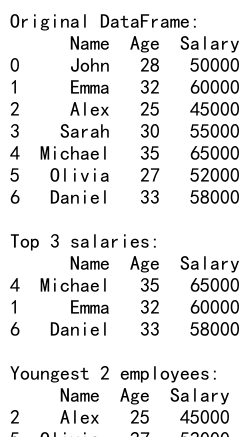
In this example, we use nlargest() to select the 3 employees with the highest salaries and nsmallest() to select the 2 youngest employees. These methods are particularly useful when you want to quickly identify extreme values in your dataset.

12. Filtering with `mask()` and `where()`

The mask() and where() methods provide another way to filter data, allowing you to replace values that don’t meet a certain condition.

import pandas as pd
import numpy as np

# Create a sample DataFrame
df = pd.DataFrame({
    'Product': ['A', 'B', 'C', 'D', 'E'],
    'Price': [10, 25, 30, 45, 50],
    'Stock': [100, 50, 75, 30, 20]
})

# Replace stock values with NaN where price is less than 30
filtered_df = df.where(df['Price'] >= 30)

# Replace price values with 0 where stock is less than 50
masked_df = df.mask(df['Stock'] < 50, {'Price': 0})

print("Original DataFrame:")
print(df)
print("\nFiltered DataFrame (using where):")
print(filtered_df)
print("\nMasked DataFrame (using mask):")
print(masked_df)

Output:

Pandas Filter

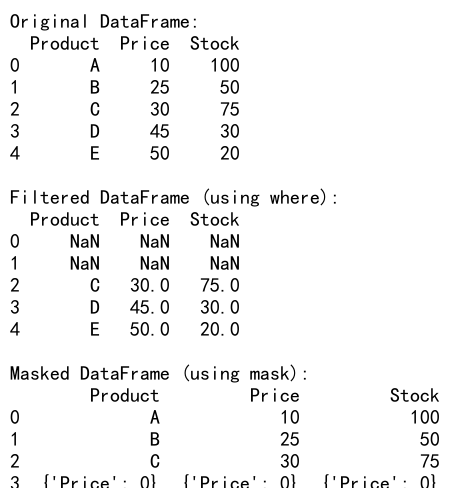
In this example, we demonstrate two filtering techniques:
1. Using where() to replace stock values with NaN where the price is less than 30
2. Using mask() to replace price values with 0 where the stock is less than 50

These methods are useful when you want to selectively modify data based on certain conditions while preserving the original DataFrame structure.

13. Filtering with `filter()` Method

The filter() method is used to select a subset of rows or columns based on their labels or a callable function.

import pandas as pd

# Create a sample DataFrame
df = pd.DataFrame({
    'A_val': [1, 2, 3],
    'B_val': [4, 5, 6],
    'C_val': [7, 8, 9],
    'D_val': [10, 11, 12],
    'E_other': [13, 14, 15]
})

# Filter columns that end with 'val'
filtered_df = df.filter(regex='val$')

# Filter columns using a list of column names
selected_columns = df.filter(items=['A_val', 'C_val', 'E_other'])

print("Original DataFrame:")
print(df)
print("\nFiltered DataFrame (columns ending with 'val'):")
print(filtered_df)
print("\nSelected columns:")
print(selected_columns)

Output:

Pandas Filter

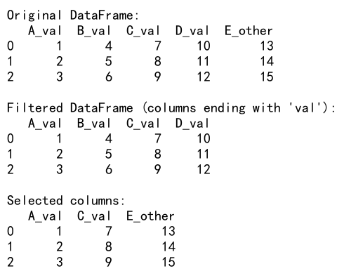
In this example, we use the filter() method in two ways:
1. To select columns that end with ‘val’ using a regular expression
2. To select specific columns by their names

This method is particularly useful when you want to select columns based on patterns in their names or when you have a list of column names you want to include.

14. Filtering with `eval()` Method

The eval() method allows you to filter DataFrames using string expressions, similar to query(), but with more flexibility and the ability to use temporary variables.

import pandas as pd

# Create a sample DataFrame
df = pd.DataFrame({
    'Name': ['John', 'Emma', 'Alex', 'Sarah', 'Michael'],
    'Age': [28, 32, 25, 30, 35],
    'Salary': [50000, 60000, 45000, 55000, 65000],
    'Department': ['Sales', 'Marketing', 'IT', 'HR', 'Finance']
})

# Filter using eval
filtered_df = df[df.eval('(Age > 30) & (Salary > 55000) | (Department == "IT")')]

print("Original DataFrame:")
print(df)
print("\nFiltered DataFrame:")
print(filtered_df)

Output:

Pandas Filter

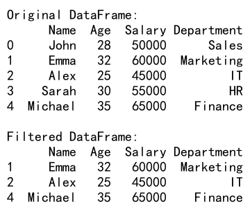
In this example, we use eval() to filter the DataFrame based on a complex condition: employees who are either over 30 years old and earn more than 55000, or who work in the IT department. The eval() method allows us to express this condition as a string, which can be more readable for complex queries.

15. Filtering with `pd.cut()` for Binning

Sometimes, you may want to filter data based on bins or categories. The pd.cut() function is useful for this purpose.

import pandas as pd

# Create a sample DataFrame
df = pd.DataFrame({
    'Name': ['John', 'Emma', 'Alex', 'Sarah', 'Michael', 'Olivia', 'Daniel'],
    'Age': [28, 32, 25, 30, 35, 27, 33],
    'Salary': [50000, 60000, 45000, 55000, 65000, 52000, 58000]
})

# Create age bins
age_bins = [0, 25, 30, 35, 100]
age_labels = ['Young', 'Adult', 'Mid-Adult', 'Senior']

df['Age_Group'] = pd.cut(df['Age'], bins=age_bins, labels=age_labels, right=False)

# Filter to get only 'Adult' and 'Mid-Adult' age groups
filtered_df = df[df['Age_Group'].isin(['Adult', 'Mid-Adult'])]

print("Original DataFrame with Age Groups:")
print(df)
print("\nFiltered DataFrame:")
print(filtered_df)

Output:

Pandas Filter

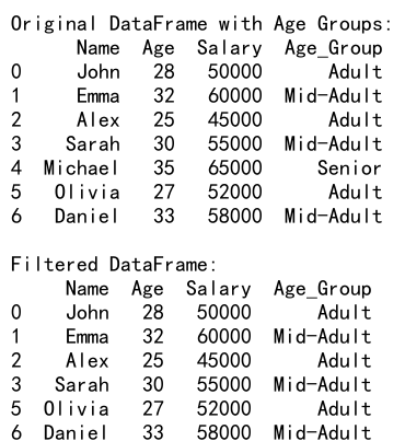
In this example, we use pd.cut() to create age groups based on specified bins. We then filter the DataFrame to include only the ‘Adult’ and ‘Mid-Adult’ age groups. This technique is useful when you want to categorize continuous data and then filter based on these categories.

16. Filtering with `groupby()` and Aggregation

Combining filtering with groupby operations allows for powerful data analysis. Here’s an example that filters groups based on aggregated values:

import pandas as pd

# Create a sample DataFrame
df = pd.DataFrame({
    'Name': ['John', 'Emma', 'Alex', 'Sarah', 'Michael', 'Olivia', 'Daniel'],
    'Department': ['Sales', 'Marketing', 'IT', 'HR', 'Sales', 'Marketing', 'IT'],
    'Salary': [50000, 60000, 45000, 55000, 65000, 52000, 58000]
})

# Group by department and calculate average salary
dept_avg_salary = df.groupby('Department')['Salary'].mean()

# Filter departments with average salary > 55000
high_paying_depts = dept_avg_salary[dept_avg_salary > 55000]

# Filter original DataFrame to include only high-paying departments
filtered_df = df[df['Department'].isin(high_paying_depts.index)]

print("Original DataFrame:")
print(df)
print("\nDepartment Average Salaries:")
print(dept_avg_salary)
print("\nHigh-Paying Departments:")
print(high_paying_depts)
print("\nFiltered DataFrame:")
print(filtered_df)

Output:

Pandas Filter

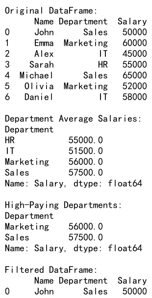
In this example, we group the DataFrame by department and calculate the average salary for each department. We then filter to find departments with an average salary above 55000, and use this to filter the original DataFrame. This approach allows us to filter based on aggregate statistics of groups.

17. Filtering with Multi-Index DataFrames

When working with multi-index DataFrames, filtering can be applied at different levels of the index hierarchy.

import pandas as pd

# Create a sample multi-index DataFrame
index = pd.MultiIndex.from_product([['A', 'B', 'C'], ['X', 'Y', 'Z']], names=['Level1', 'Level2'])
df = pd.DataFrame(index=index, columns=['Value1', 'Value2'], data=range(18)).reset_index()
df['Value1'] = [10, 20, 30, 40, 50, 60, 70, 80, 90] * 2
df.set_index(['Level1', 'Level2'], inplace=True)

# Filter rows where Level1 is 'A' or 'B' and Value1 > 30
filtered_df = df.loc[(df.index.get_level_values('Level1').isin(['A', 'B'])) & (df['Value1'] > 30)]

print("Original Multi-Index DataFrame:")
print(df)
print("\nFiltered DataFrame:")
print(filtered_df)

In this example, we create a multi-index DataFrame and demonstrate how to filter it based on conditions applied to both index levels and data columns. We select rows where the first level of the index is either ‘A’ or ‘B’, and the ‘Value1’ column is greater than 30.

18. Filtering with `pd.Timestamp` for Date Ranges

When working with datetime data, pd.Timestamp can be used for precise filtering of date ranges.

import pandas as pd

# Create a sample DataFrame with date index
date_range = pd.date_range(start='2023-01-01', end='2023-12-31', freq='D')
df = pd.DataFrame(index=date_range, columns=['Value'], data=range(365))

# Filter data between two specific dates
start_date = pd.Timestamp('2023-03-15')
end_date = pd.Timestamp('2023-04-15')

filtered_df = df.loc[start_date:end_date]

print("Original DataFrame (first 5 rows):")
print(df.head())
print("\nFiltered DataFrame:")
print(filtered_df)

Output:

Pandas Filter

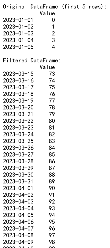
In this example, we create a DataFrame with a date index spanning the year 2023. We then use pd.Timestamp to define specific start and end dates, and filter the DataFrame to include only the data within this date range.

Pandas Filter Conclusion

Filtering is a fundamental operation in data analysis with pandas, and as we’ve seen, there are numerous methods and techniques available to suit different needs and data structures. From simple boolean indexing to complex multi-index slicing, pandas provides a rich set of tools for data filtering.

Key points to remember:
1. Boolean indexing is the most common and versatile method for filtering.
2. The loc and iloc accessors provide powerful ways to select data based on labels or integer positions.
3. The query() and eval() methods offer a concise syntax for complex filtering conditions.
4. String methods and regular expressions can be used for text-based filtering.
5. Date and time filtering can be achieved using various datetime accessors and functions.
6. For multi-index DataFrames, techniques like IndexSlice can be very useful.
7. Custom functions can be used with apply() for complex filtering logic.

As you work with different datasets and analysis requirements, you’ll likely find yourself using a combination of these filtering techniques. The key is to choose the method that best fits your specific data structure and filtering needs, always keeping in mind the readability and efficiency of your code.

Remember that filtering is often just the first step in a data analysis pipeline. After filtering your data, you might proceed with further analysis, visualization, or modeling tasks. Mastering these filtering techniques will give you the ability to quickly and efficiently focus on the most relevant parts of your data, setting a strong foundation for all your subsequent analysis tasks.

Pandas Filter

Pandas Filter

1. Introduction to Pandas Filtering

2. Boolean Indexing

2.1 Simple Boolean Indexing

2.2 Combining Multiple Conditions

3. Using `loc` and `iloc` for Filtering

3.1 Filtering with `loc`

3.2 Filtering with `iloc`

4. Using the `query()` Method

5. Filtering with String Methods

6. Filtering with Regular Expressions

7. Filtering Date and Time Data

8. Filtering with `isin()` Method

9. Filtering with `between()` Method

10. Filtering with Custom Functions

11. Filtering with `nsmallest()` and `nlargest()`

12. Filtering with `mask()` and `where()`

13. Filtering with `filter()` Method

14. Filtering with `eval()` Method

15. Filtering with `pd.cut()` for Binning

16. Filtering with `groupby()` and Aggregation

17. Filtering with Multi-Index DataFrames

18. Filtering with `pd.Timestamp` for Date Ranges

Pandas Filter Conclusion

Pandas Articles

Bookmarks

Top

Pandas Filter

1. Introduction to Pandas Filtering

2. Boolean Indexing

2.1 Simple Boolean Indexing

2.2 Combining Multiple Conditions

3. Using loc and iloc for Filtering

3.1 Filtering with loc

3.2 Filtering with iloc

4. Using the query() Method

5. Filtering with String Methods

6. Filtering with Regular Expressions

7. Filtering Date and Time Data

8. Filtering with isin() Method

9. Filtering with between() Method

10. Filtering with Custom Functions

11. Filtering with nsmallest() and nlargest()

12. Filtering with mask() and where()

13. Filtering with filter() Method

14. Filtering with eval() Method

15. Filtering with pd.cut() for Binning

16. Filtering with groupby() and Aggregation

17. Filtering with Multi-Index DataFrames

18. Filtering with pd.Timestamp for Date Ranges

Pandas Filter Conclusion

Pandas Articles

Bookmarks

Top

3. Using `loc` and `iloc` for Filtering

3.1 Filtering with `loc`

3.2 Filtering with `iloc`

4. Using the `query()` Method

8. Filtering with `isin()` Method

9. Filtering with `between()` Method

11. Filtering with `nsmallest()` and `nlargest()`

12. Filtering with `mask()` and `where()`

13. Filtering with `filter()` Method

14. Filtering with `eval()` Method

15. Filtering with `pd.cut()` for Binning

16. Filtering with `groupby()` and Aggregation

18. Filtering with `pd.Timestamp` for Date Ranges