Pandas Filter DataFrame

Pandas Filter DataFrame

Pandas is a powerful data manipulation library in Python, and one of its most essential features is the ability to filter DataFrames. Filtering allows you to select specific rows or columns based on certain conditions, enabling you to focus on the data that matters most for your analysis. In this comprehensive guide, we’ll explore various methods and techniques for filtering DataFrames in Pandas, providing detailed explanations and numerous code examples to help you master this crucial skill.

1. Introduction to DataFrame Filtering

Before diving into the specifics of filtering, let’s briefly review what a DataFrame is and why filtering is important. A DataFrame is a two-dimensional labeled data structure in Pandas, similar to a spreadsheet or SQL table. It consists of rows and columns, where each column can have a different data type.

Filtering a DataFrame is the process of selecting a subset of data based on specific criteria. This is crucial for data analysis and manipulation tasks, as it allows you to:

1. Focus on relevant data
2. Remove outliers or unwanted information
3. Perform operations on specific subsets of your data
4. Prepare data for visualization or further analysis

Now, let’s explore the various methods for filtering DataFrames in Pandas.

2. Boolean Indexing

Boolean indexing is one of the most common and versatile methods for filtering DataFrames. It involves creating a boolean mask (an array of True/False values) and using it to select rows that meet certain conditions.

Let’s start with a simple example:

import pandas as pd
import numpy as np

# Create a sample DataFrame
df = pd.DataFrame({
    'Name': ['John', 'Emma', 'Alex', 'Sarah', 'Michael'],
    'Age': [28, 32, 24, 35, 29],
    'City': ['New York', 'London', 'Paris', 'Tokyo', 'Sydney'],
    'Salary': [50000, 75000, 45000, 80000, 60000]
})

# Filter rows where Age is greater than 30
filtered_df = df[df['Age'] > 30]

print("Original DataFrame:")
print(df)
print("\nFiltered DataFrame:")
print(filtered_df)

Output:

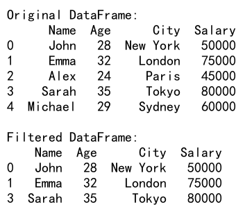
In this example, we create a boolean mask df['Age'] > 30, which returns a Series of True/False values. We then use this mask to index the DataFrame, selecting only the rows where the condition is True.

You can also combine multiple conditions using logical operators:

import pandas as pd

# Create a sample DataFrame
df = pd.DataFrame({
    'Name': ['John', 'Emma', 'Alex', 'Sarah', 'Michael'],
    'Age': [28, 32, 24, 35, 29],
    'City': ['New York', 'London', 'Paris', 'Tokyo', 'Sydney'],
    'Salary': [50000, 75000, 45000, 80000, 60000]
})

# Filter rows where Age is greater than 30 and Salary is less than 80000
filtered_df = df[(df['Age'] > 30) & (df['Salary'] < 80000)]

print("Original DataFrame:")
print(df)
print("\nFiltered DataFrame:")
print(filtered_df)

Output:

In this example, we use the & operator to combine two conditions. Note that each condition must be enclosed in parentheses when using logical operators.

3. Using the .loc[] Accessor

The .loc[] accessor is another powerful method for filtering DataFrames. It allows you to select data based on labels or boolean arrays.

Here’s an example of using .loc[] with a boolean mask:

import pandas as pd

# Create a sample DataFrame
df = pd.DataFrame({
    'Name': ['John', 'Emma', 'Alex', 'Sarah', 'Michael'],
    'Age': [28, 32, 24, 35, 29],
    'City': ['New York', 'London', 'Paris', 'Tokyo', 'Sydney'],
    'Salary': [50000, 75000, 45000, 80000, 60000]
})

# Filter rows where City is 'London' or 'Tokyo'
filtered_df = df.loc[df['City'].isin(['London', 'Tokyo'])]

print("Original DataFrame:")
print(df)
print("\nFiltered DataFrame:")
print(filtered_df)

Output:

In this example, we use the .isin() method to check if the ‘City’ column contains either ‘London’ or ‘Tokyo’. The resulting boolean mask is then used with .loc[] to select the matching rows.

You can also use .loc[] to select specific columns along with filtered rows:

import pandas as pd

# Create a sample DataFrame
df = pd.DataFrame({
    'Name': ['John', 'Emma', 'Alex', 'Sarah', 'Michael'],
    'Age': [28, 32, 24, 35, 29],
    'City': ['New York', 'London', 'Paris', 'Tokyo', 'Sydney'],
    'Salary': [50000, 75000, 45000, 80000, 60000]
})

# Filter rows where Age is greater than 30 and select only 'Name' and 'Salary' columns
filtered_df = df.loc[df['Age'] > 30, ['Name', 'Salary']]

print("Original DataFrame:")
print(df)
print("\nFiltered DataFrame:")
print(filtered_df)

Output:

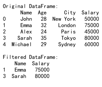
This example demonstrates how to combine row filtering with column selection using .loc[].

4. Using the .query() Method

The .query() method provides a concise way to filter DataFrames using a string expression. This can be particularly useful when dealing with complex conditions or when you want to make your code more readable.

Here’s an example of using .query():

import pandas as pd

# Create a sample DataFrame
df = pd.DataFrame({
    'Name': ['John', 'Emma', 'Alex', 'Sarah', 'Michael'],
    'Age': [28, 32, 24, 35, 29],
    'City': ['New York', 'London', 'Paris', 'Tokyo', 'Sydney'],
    'Salary': [50000, 75000, 45000, 80000, 60000]
})

# Filter rows where Age is between 25 and 35, and Salary is greater than 60000
filtered_df = df.query('25 <= Age <= 35 and Salary > 60000')

print("Original DataFrame:")
print(df)
print("\nFiltered DataFrame:")
print(filtered_df)

Output:

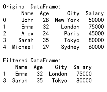
The .query() method accepts a string expression that defines the filtering conditions. In this example, we filter rows where the Age is between 25 and 35 (inclusive) and the Salary is greater than 60000.

You can also use variables in your query by prefixing them with @:

import pandas as pd

# Create a sample DataFrame
df = pd.DataFrame({
    'Name': ['John', 'Emma', 'Alex', 'Sarah', 'Michael'],
    'Age': [28, 32, 24, 35, 29],
    'City': ['New York', 'London', 'Paris', 'Tokyo', 'Sydney'],
    'Salary': [50000, 75000, 45000, 80000, 60000]
})

# Define variables for filtering
min_age = 30
max_salary = 70000

# Filter rows using variables
filtered_df = df.query('Age >= @min_age and Salary <= @max_salary')

print("Original DataFrame:")
print(df)
print("\nFiltered DataFrame:")
print(filtered_df)

Output:

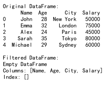
This example demonstrates how to use variables in a .query() expression by prefixing them with @.

5. Filtering with String Methods

Pandas provides string methods that can be applied to columns containing string data. These methods are accessible through the .str accessor and can be used for filtering based on string patterns or operations.

Here’s an example of filtering based on a string pattern:

import pandas as pd

# Create a sample DataFrame
df = pd.DataFrame({
    'Name': ['John Smith', 'Emma Johnson', 'Alex Brown', 'Sarah Davis', 'Michael Wilson'],
    'Email': ['[email protected]', '[email protected]', '[email protected]', '[email protected]', '[email protected]']
})

# Filter rows where the email contains 'pandasdataframe.com'
filtered_df = df[df['Email'].str.contains('pandasdataframe.com')]

print("Original DataFrame:")
print(df)
print("\nFiltered DataFrame:")
print(filtered_df)

Output:

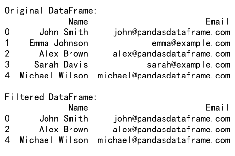
In this example, we use the .str.contains() method to filter rows where the ‘Email’ column contains the string ‘pandasdataframe.com’.

You can also use regular expressions with string methods:

import pandas as pd

# Create a sample DataFrame
df = pd.DataFrame({
    'Name': ['John Smith', 'Emma Johnson', 'Alex Brown', 'Sarah Davis', 'Michael Wilson'],
    'Email': ['[email protected]', '[email protected]', '[email protected]', '[email protected]', '[email protected]']
})

# Filter rows where the name starts with 'J' or 'M'
filtered_df = df[df['Name'].str.match(r'^[JM]')]

print("Original DataFrame:")
print(df)
print("\nFiltered DataFrame:")
print(filtered_df)

Output:

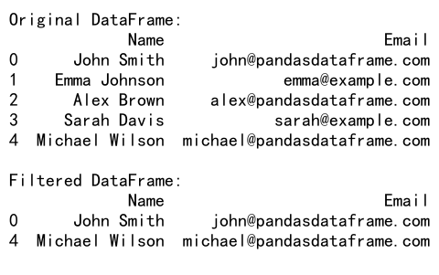
This example uses the .str.match() method with a regular expression to filter rows where the ‘Name’ column starts with either ‘J’ or ‘M’.

6. Filtering with DateTime Methods

When working with datetime data, Pandas provides specific methods for filtering based on date and time conditions. These methods are accessible through the .dt accessor.

Let’s look at an example:

import pandas as pd

# Create a sample DataFrame with datetime data
df = pd.DataFrame({
    'Date': pd.date_range(start='2023-01-01', end='2023-12-31', freq='D'),
    'Value': range(365)
})

# Filter rows for the month of June
filtered_df = df[df['Date'].dt.month == 6]

print("Original DataFrame:")
print(df)
print("\nFiltered DataFrame:")
print(filtered_df)

Output:

In this example, we create a DataFrame with a full year of daily data and then filter it to show only the rows for the month of June using the .dt.month accessor.

You can combine multiple datetime conditions:

import pandas as pd

# Create a sample DataFrame with datetime data
df = pd.DataFrame({
    'Date': pd.date_range(start='2023-01-01', end='2023-12-31', freq='D'),
    'Value': range(365)
})

# Filter rows for weekends in the first quarter
filtered_df = df[(df['Date'].dt.quarter == 1) & (df['Date'].dt.dayofweek.isin([5, 6]))]

print("Original DataFrame:")
print(df)
print("\nFiltered DataFrame:")
print(filtered_df)

Output:

This example filters the DataFrame to show only weekend days (Saturday and Sunday) in the first quarter of the year.

7. Filtering with Categorical Data

When working with categorical data, you can use the cat accessor to perform filtering operations. This is particularly useful when dealing with ordered categories.

Here’s an example:

import pandas as pd

# Create a sample DataFrame with categorical data
df = pd.DataFrame({
    'Name': ['John', 'Emma', 'Alex', 'Sarah', 'Michael'],
    'Education': pd.Categorical(['High School', 'Bachelor', 'Master', 'PhD', 'Bachelor'],
                                categories=['High School', 'Bachelor', 'Master', 'PhD'],
                                ordered=True)
})

# Filter rows where Education is higher than Bachelor
filtered_df = df[df['Education'].cat.codes > df['Education'].cat.categories.get_loc('Bachelor')]

print("Original DataFrame:")
print(df)
print("\nFiltered DataFrame:")
print(filtered_df)

Output:

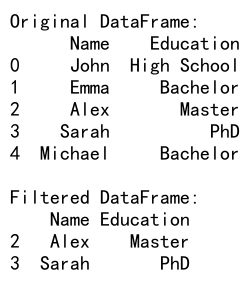
In this example, we create a DataFrame with an ordered categorical column ‘Education’. We then filter the DataFrame to show only rows where the education level is higher than ‘Bachelor’.

You can also use the .isin() method with categorical data:

import pandas as pd

# Create a sample DataFrame with categorical data
df = pd.DataFrame({
    'Name': ['John', 'Emma', 'Alex', 'Sarah', 'Michael'],
    'Department': pd.Categorical(['Sales', 'Marketing', 'IT', 'HR', 'Finance'])
})

# Filter rows for specific departments
filtered_df = df[df['Department'].isin(['Sales', 'Marketing', 'IT'])]

print("Original DataFrame:")
print(df)
print("\nFiltered DataFrame:")
print(filtered_df)

Output:

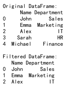
This example demonstrates how to filter rows based on specific categories using the .isin() method.

8. Advanced Filtering Techniques

Now that we’ve covered the basics, let’s explore some more advanced filtering techniques that can be useful in complex data analysis scenarios.

8.1 Filtering with Custom Functions

You can use custom functions to create complex filtering conditions that are not easily expressed using standard comparison operators.

Here’s an example:

import pandas as pd

# Create a sample DataFrame
df = pd.DataFrame({
    'Name': ['John', 'Emma', 'Alex', 'Sarah', 'Michael'],
    'Age': [28, 32, 24, 35, 29],
    'City': ['New York', 'London', 'Paris', 'Tokyo', 'Sydney'],
    'Salary': [50000, 75000, 45000, 80000, 60000]
})

# Define a custom filtering function
def complex_condition(row):
    return (row['Age'] > 30 and row['Salary'] > 70000) or (row['City'] == 'New York' and row['Age'] < 30)

# Apply the custom function to filter the DataFrame
filtered_df = df[df.apply(complex_condition, axis=1)]

print("Original DataFrame:")
print(df)
print("\nFiltered DataFrame:")
print(filtered_df)

Output:

In this example, we define a custom function complex_condition that checks for a combination of conditions. We then use df.apply() to apply this function to each row of the DataFrame, creating a boolean mask for filtering.

8.2 Filtering with MultiIndex

When working with MultiIndex DataFrames, you can filter based on multiple levels of the index.

Here’s an example:

import pandas as pd
import numpy as np

# Create a sample MultiIndex DataFrame
index = pd.MultiIndex.from_product([['A', 'B', 'C'], [2021, 2022, 2023]], names=['Category', 'Year'])
df = pd.DataFrame(np.random.randn(9, 2), index=index, columns=['Value1', 'Value2'])

# Filter rows where Category is 'A' or 'B' and Year is 2022 or 2023
filtered_df = df.loc[(df.index.get_level_values('Category').isin(['A', 'B'])) & 
                     (df.index.get_level_values('Year').isin([2022, 2023]))]

print("Original DataFrame:")
print(df)
print("\nFiltered DataFrame:")
print(filtered_df)

Output:

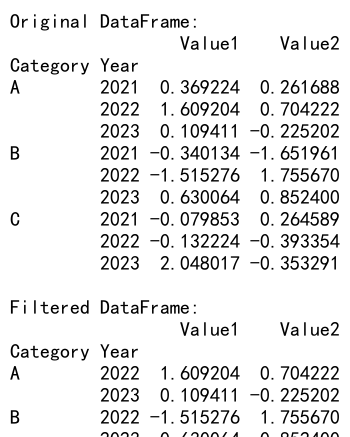
This example demonstrates how to filter a MultiIndex DataFrame based on conditions applied to different levels of the index.

8.3 Filtering with .where() and .mask()

The .where() and .mask() methods provide alternative ways to filter DataFrames, allowing you to replace values that don’t meet certain conditions.

Here’s an example using .where():

import pandas as pd
import numpy as np

# Create a sample DataFrame
df = pd.DataFrame({
    'A': [1, 2, 3, 4, 5],
    'B': [10, 20, 30, 40, 50],
    'C': [100, 200, 300, 400, 500]
})

# Replace values in column 'A' with NaN if they are less than 3
filtered_df = df.where(df['A'] >= 3)

print("Original DataFrame:")
print(df)
print("\nFiltered DataFrame:")
print(filtered_df)

Output:

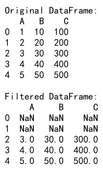
In this example, .where() replaces values in the DataFrame with NaN if they don’t meet the specified condition.

And here’s an example using .mask():

import pandas as pd
import numpy as np

# Create a sample DataFrame
df = pd.DataFrame({
    'A': [1, 2, 3, 4, 5],
    'B': [10, 20, 30, 40, 50],
    'C': [100, 200, 300, 400, 500]
})

# Replace values in column 'A' with NaN if they are greater than or equal to 3
filtered_df = df.mask(df['A'] >= 3)

print("Original DataFrame:")
print(df)
print("\nFiltered DataFrame:")
print(filtered_df)

Output:

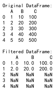
The .mask() method is the inverse of .where(). It replaces values with NaN if they meet the specified condition.

9. Handling Missing Data

When filtering DataFrames, you often need to deal with missing data. Pandas provides several methods to handle NaN (Not a Number) values.

9.1 Filtering out NaN values

To remove rows with NaN values, you can use the .dropna() method:

import pandas as pd
import numpy as np

# Create a sample DataFrame with some NaN values
df = pd.DataFrame({
    'A': [1, 2, np.nan, 4, 5],
    'B': [10, np.nan, 30, 40, 50],
    'C': [100, 200, 300, np.nan, 500]
})

# Remove rows with any NaN values
filtered_df = df.dropna()

print("Original DataFrame:")
print(df)
print("\nFiltered DataFrame:")
print(filtered_df)

Output:

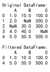
This example removes all rows that contain at least one NaN value.

9.2 Filtering based on NaN values

You can also filter rows based on whether they contain NaN values:

import pandas as pd
import numpy as np

# Create a sample DataFrame with some NaN values
df = pd.DataFrame({
    'A': [1, 2, np.nan, 4, 5],
    'B': [10, np.nan, 30, 40, 50],
    'C': [100, 200, 300, np.nan, 500]
})

# Keep only rows where column 'A' is not NaN
filtered_df = df[df['A'].notna()]

print("Original DataFrame:")
print(df)
print("\nFiltered DataFrame:")
print(filtered_df)

Output:

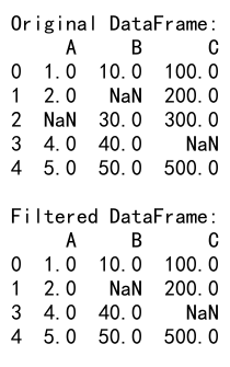
This example keeps only the rows where column ‘A’ is not NaN.

10. Combining Multiple Filters

In real-world scenarios, you often need to apply multiple filters to your data. Pandas allows you to combine filters using logical operators.

10.1 Using & (AND) operator

To combine multiple conditions where all must be true, use the & operator:

import pandas as pd

# Create a sample DataFrame
df = pd.DataFrame({
    'Name': ['John', 'Emma', 'Alex', 'Sarah', 'Michael'],
    'Age': [28, 32, 24, 35, 29],
    'City': ['New York', 'London', 'Paris', 'Tokyo', 'Sydney'],
    'Salary': [50000, 75000, 45000, 80000, 60000]
})

# Filter rows where Age > 30 AND City is 'London'
filtered_df = df[(df['Age'] > 30) & (df['City'] == 'London')]

print("Original DataFrame:")
print(df)
print("\nFiltered DataFrame:")
print(filtered_df)

Output:

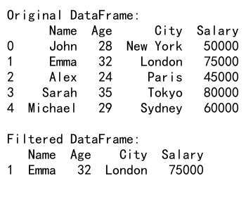
This example filters the DataFrame to show only rows where the age is greater than 30 and the city is London.

10.2 Using | (OR) operator

To combine multiple conditions where at least one must be true, use the | operator:

import pandas as pd

# Create a sample DataFrame
df = pd.DataFrame({
    'Name': ['John', 'Emma', 'Alex', 'Sarah', 'Michael'],
    'Age': [28, 32, 24, 35, 29],
    'City': ['New York', 'London', 'Paris', 'Tokyo', 'Sydney'],
    'Salary': [50000, 75000, 45000, 80000, 60000]
})

# Filter rows where Age < 25 OR Salary > 70000
filtered_df = df[(df['Age'] < 25) | (df['Salary'] > 70000)]

print("Original DataFrame:")
print(df)
print("\nFiltered DataFrame:")
print(filtered_df)

Output:

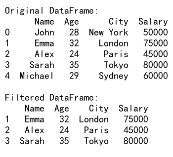
This example filters the DataFrame to show rows where either the age is less than 25 or the salary is greater than 70000.

11. Filtering and Updating Data

Sometimes you may want to filter data and then update the values that meet certain conditions. Pandas allows you to do this efficiently.

11.1 Updating filtered data

Here’s an example of updating values in a filtered DataFrame:

import pandas as pd

# Create a sample DataFrame
df = pd.DataFrame({
    'Name': ['John', 'Emma', 'Alex', 'Sarah', 'Michael'],
    'Age': [28, 32, 24, 35, 29],
    'City': ['New York', 'London', 'Paris', 'Tokyo', 'Sydney'],
    'Salary': [50000, 75000, 45000, 80000, 60000]
})

# Increase salary by 10% for employees older than 30
df.loc[df['Age'] > 30, 'Salary'] *= 1.1

print("Updated DataFrame:")
print(df)

Output:

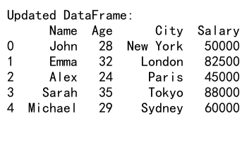
This example increases the salary by 10% for employees older than 30.

11.2 Conditional updating with .where()

You can also use the .where() method to update values conditionally:

import pandas as pd

# Create a sample DataFrame
df = pd.DataFrame({
    'Name': ['John', 'Emma', 'Alex', 'Sarah', 'Michael'],
    'Age': [28, 32, 24, 35, 29],
    'City': ['New York', 'London', 'Paris', 'Tokyo', 'Sydney'],
    'Salary': [50000, 75000, 45000, 80000, 60000]
})

# Set salary to 100000 for employees in New York, keep others unchanged
df['Salary'] = df['Salary'].where(df['City'] != 'New York', 100000)

print("Updated DataFrame:")
print(df)

Output:

This example sets the salary to 100000 for employees in New York while keeping other salaries unchanged.

12. Performance Considerations

When working with large DataFrames, the performance of filtering operations becomes crucial. Here are some tips to optimize your filtering operations:

12.1 Use vectorized operations

Whenever possible, use vectorized operations instead of applying functions to each row. Vectorized operations are much faster, especially for large DataFrames.

import pandas as pd
import numpy as np

# Create a large sample DataFrame
df = pd.DataFrame({
    'A': np.random.randn(1000000),
    'B': np.random.randn(1000000),
    'C': np.random.choice(['X', 'Y', 'Z'], 1000000)
})

# Slow method (avoid for large DataFrames)
# filtered_df = df[df.apply(lambda row: row['A'] > 0 and row['B'] < 0, axis=1)]

# Fast method (vectorized)
filtered_df = df[(df['A'] > 0) & (df['B'] < 0)]

print("Filtered DataFrame shape:", filtered_df.shape)

Output:

This example demonstrates the vectorized approach to filtering, which is much faster for large DataFrames.

12.2 Use .query() for complex conditions

For complex filtering conditions, especially those involving multiple columns, the .query() method can be more efficient than boolean indexing:

import pandas as pd
import numpy as np

# Create a large sample DataFrame
df = pd.DataFrame({
    'A': np.random.randn(1000000),
    'B': np.random.randn(1000000),
    'C': np.random.choice(['X', 'Y', 'Z'], 1000000)
})

# Using .query() for complex conditions
filtered_df = df.query('A > 0 and B < 0 and C == "X"')

print("Filtered DataFrame shape:", filtered_df.shape)

Output:

The .query() method can be more efficient for complex conditions, especially when dealing with large DataFrames.

13. Filtering with Index

You can also filter DataFrames based on their index values. This is particularly useful when working with time series data or when your index contains meaningful information.

import pandas as pd

# Create a sample DataFrame with a date index
df = pd.DataFrame({
    'Value': range(100, 131)
}, index=pd.date_range(start='2023-01-01', end='2023-01-31'))

# Filter rows for a specific date range
filtered_df = df.loc['2023-01-15':'2023-01-20']

print("Original DataFrame:")
print(df)
print("\nFiltered DataFrame:")
print(filtered_df)

Output:

This example filters the DataFrame to show only rows within a specific date range using the index.

14. Pandas Filter DataFrame Conclusion

Filtering DataFrames is a fundamental skill in data analysis with Pandas. We’ve covered a wide range of techniques, from basic boolean indexing to advanced methods like .query() and custom functions. Here’s a summary of the key points:

1. Boolean indexing is the most common method for filtering DataFrames.
2. The .loc[] accessor provides a powerful way to filter rows and select columns simultaneously.
3. The .query() method offers a concise syntax for complex filtering conditions.
4. String methods (.str) and datetime methods (.dt) provide specialized filtering capabilities for string and datetime data.
5. Categorical data can be filtered using the .cat accessor.
6. Advanced techniques like custom functions and MultiIndex filtering allow for more complex data selection.
7. Methods like .where() and .mask() offer alternative ways to filter and update data.
8. Handling missing data is crucial when filtering DataFrames.
9. Multiple filters can be combined using logical operators (&, |).
10. Performance considerations are important when working with large DataFrames.

By mastering these filtering techniques, you’ll be well-equipped to handle a wide variety of data analysis tasks in Pandas. Remember to choose the most appropriate method based on your specific use case and data structure. Happy data wrangling!