Mastering Pandas GroupBy Rank

Mastering Pandas GroupBy Rank

Pandas groupby rank is a powerful feature in the pandas library that allows you to perform ranking operations within groups of data. This functionality is essential for data analysts and scientists who need to analyze and manipulate large datasets efficiently. In this comprehensive guide, we’ll explore the ins and outs of pandas groupby rank, providing detailed explanations and practical examples to help you master this important tool.

Understanding Pandas GroupBy Rank

Pandas groupby rank combines two key concepts in pandas: groupby and rank. The groupby operation allows you to split your data into groups based on one or more columns, while the rank function assigns ranks to values within a series or dataframe. When used together, pandas groupby rank enables you to rank values within specific groups of your data.

Let’s start with a simple example to illustrate the basic concept of pandas groupby rank:

import pandas as pd

# Create a sample dataframe
df = pd.DataFrame({
    'name': ['Alice', 'Bob', 'Charlie', 'David', 'Alice', 'Bob'],
    'score': [85, 92, 78, 95, 88, 90],
    'subject': ['Math', 'Math', 'Science', 'Science', 'Science', 'Math']
})

# Apply groupby rank
df['rank'] = df.groupby('subject')['score'].rank(method='dense', ascending=False)

print(df)

Output:

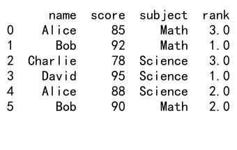
In this example, we create a dataframe with student names, scores, and subjects. We then use pandas groupby rank to rank the scores within each subject group. The method='dense' parameter ensures that ties are assigned the same rank, and ascending=False ranks the highest scores first.

The Power of Pandas GroupBy Rank in Data Analysis

Pandas groupby rank is an invaluable tool for various data analysis tasks. It allows you to:

1. Identify top performers within groups
2. Calculate percentiles within categories
3. Create custom rankings based on multiple criteria
4. Analyze trends and patterns across different segments of your data

Let’s explore some more advanced applications of pandas groupby rank:

import pandas as pd
import numpy as np

# Create a larger dataset
np.random.seed(42)
df = pd.DataFrame({
    'department': np.random.choice(['Sales', 'Marketing', 'IT'], 1000),
    'employee': [f'emp_{i}' for i in range(1000)],
    'sales': np.random.randint(1000, 10000, 1000),
    'performance': np.random.uniform(1, 5, 1000)
})

# Rank employees by sales within each department
df['sales_rank'] = df.groupby('department')['sales'].rank(method='min', ascending=False)

# Rank employees by performance within each department
df['performance_rank'] = df.groupby('department')['performance'].rank(method='dense')

# Calculate percentile rank for sales within each department
df['sales_percentile'] = df.groupby('department')['sales'].rank(pct=True)

print(df.head(10))

Output:

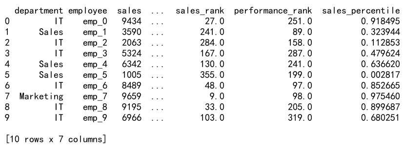
In this example, we create a larger dataset with employee information from different departments. We then use pandas groupby rank to:

1. Rank employees by sales within each department
2. Rank employees by performance within each department
3. Calculate the percentile rank for sales within each department

This demonstrates how pandas groupby rank can be used to analyze employee performance across different dimensions and departments.

Advanced Techniques with Pandas GroupBy Rank

Now that we’ve covered the basics, let’s explore some more advanced techniques using pandas groupby rank:

Multi-level Grouping

Pandas groupby rank supports multi-level grouping, allowing you to rank data based on multiple criteria:

import pandas as pd

# Create a sample dataframe
df = pd.DataFrame({
    'name': ['Alice', 'Bob', 'Charlie', 'David', 'Alice', 'Bob'] * 2,
    'year': [2022, 2022, 2022, 2022, 2023, 2023] * 2,
    'quarter': [1, 1, 2, 2, 1, 1, 2, 2, 1, 1, 2, 2],
    'sales': [10000, 12000, 9000, 11000, 11000, 13000, 9500, 12000, 10500, 12500, 9800, 11500]
})

# Apply multi-level groupby rank
df['rank'] = df.groupby(['year', 'quarter'])['sales'].rank(method='dense', ascending=False)

print(df)

Output:

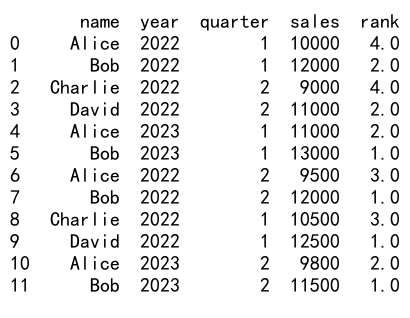
In this example, we rank sales performance within each year and quarter combination, allowing for a more granular analysis of employee performance over time.

Custom Ranking Functions

Pandas groupby rank also allows you to use custom ranking functions for more complex ranking scenarios:

import pandas as pd

# Create a sample dataframe
df = pd.DataFrame({
    'name': ['Alice', 'Bob', 'Charlie', 'David', 'Eve'],
    'sales': [100000, 120000, 90000, 110000, 95000],
    'customer_satisfaction': [4.5, 4.2, 4.8, 4.0, 4.6]
})

# Define a custom ranking function
def custom_rank(group):
    return (0.7 * group['sales'].rank(ascending=False) + 
            0.3 * group['customer_satisfaction'].rank(ascending=False))

# Apply custom ranking
df['overall_rank'] = df.groupby(df.index).apply(custom_rank)

print(df)

In this example, we create a custom ranking function that combines sales performance and customer satisfaction scores with different weights. This allows for more nuanced rankings that take multiple factors into account.

Handling Ties in Pandas GroupBy Rank

When working with pandas groupby rank, you’ll often encounter situations where multiple values within a group are tied. Pandas provides several methods for handling ties:

1. ‘average’: Assign the average rank to tied values
2. ‘min’: Assign the minimum rank to tied values
3. ‘max’: Assign the maximum rank to tied values
4. ‘first’: Assign ranks based on the order they appear in the data
5. ‘dense’: Assign ranks without gaps between tied values

Let’s explore these methods with an example:

import pandas as pd

# Create a sample dataframe
df = pd.DataFrame({
    'group': ['A', 'A', 'A', 'B', 'B', 'B'],
    'value': [10, 10, 20, 30, 30, 40]
})

# Apply different ranking methods
for method in ['average', 'min', 'max', 'first', 'dense']:
    df[f'rank_{method}'] = df.groupby('group')['value'].rank(method=method)

print(df)

Output:

This example demonstrates how different ranking methods handle ties within groups. Understanding these methods is crucial for choosing the appropriate ranking approach for your specific data analysis needs.

Percentile Ranking with Pandas GroupBy Rank

Percentile ranking is a powerful technique for understanding the relative position of values within a group. Pandas groupby rank makes it easy to calculate percentile ranks:

import pandas as pd
import numpy as np

# Create a sample dataframe
np.random.seed(42)
df = pd.DataFrame({
    'category': np.random.choice(['A', 'B', 'C'], 1000),
    'value': np.random.normal(100, 20, 1000)
})

# Calculate percentile ranks within each category
df['percentile_rank'] = df.groupby('category')['value'].rank(pct=True)

# Create bins based on percentile ranks
df['percentile_bin'] = pd.cut(df['percentile_rank'], bins=[0, 0.25, 0.5, 0.75, 1],
                              labels=['Bottom 25%', '25-50%', '50-75%', 'Top 25%'])

print(df.head(10))

Output:

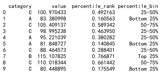
In this example, we calculate percentile ranks for values within each category and then create bins based on these percentile ranks. This approach is useful for identifying top performers, underperformers, and average performers within different groups.

Combining Pandas GroupBy Rank with Other Pandas Operations

Pandas groupby rank becomes even more powerful when combined with other pandas operations. Let’s explore some examples:

Filtering Based on Ranks

import pandas as pd

# Create a sample dataframe
df = pd.DataFrame({
    'store': ['A', 'A', 'B', 'B', 'C', 'C'] * 2,
    'product': ['X', 'Y', 'X', 'Y', 'X', 'Y'] * 2,
    'sales': [100, 150, 200, 120, 80, 90, 110, 160, 190, 130, 85, 95]
})

# Rank products within each store
df['rank'] = df.groupby('store')['sales'].rank(ascending=False)

# Filter to keep only top 2 products for each store
top_products = df[df['rank'] <= 2]

print(top_products)

Output:

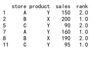
This example demonstrates how to use pandas groupby rank to identify and filter the top-performing products in each store.

Calculating Rank Changes Over Time

import pandas as pd

# Create a sample dataframe
df = pd.DataFrame({
    'date': pd.date_range(start='2023-01-01', periods=10, freq='D'),
    'product': ['A', 'B', 'C'] * 3 + ['A'],
    'sales': [100, 120, 90, 110, 130, 95, 105, 125, 85, 115]
})

# Calculate daily ranks
df['daily_rank'] = df.groupby('date')['sales'].rank(ascending=False)

# Calculate rank changes
df['rank_change'] = df.groupby('product')['daily_rank'].diff()

print(df)

Output:

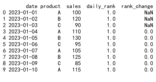
This example shows how to use pandas groupby rank to calculate daily rankings and track rank changes for products over time.

Optimizing Performance with Pandas GroupBy Rank

When working with large datasets, optimizing the performance of pandas groupby rank operations becomes crucial. Here are some tips to improve efficiency:

1. Use appropriate data types: Ensure that your columns have the correct data types to minimize memory usage and improve performance.

2. Leverage vectorized operations: Whenever possible, use vectorized operations instead of apply functions or loops.

3. Consider using categorical data: For columns with a limited number of unique values, converting them to categorical data can improve memory usage and performance.

4. Use query() for filtering: When filtering large dataframes, use the query() method instead of boolean indexing for better performance.

Let’s see an example that incorporates these optimization techniques:

import pandas as pd
import numpy as np

# Create a large sample dataframe
np.random.seed(42)
df = pd.DataFrame({
    'category': np.random.choice(['A', 'B', 'C', 'D', 'E'], 1_000_000),
    'subcategory': np.random.choice(['X', 'Y', 'Z'], 1_000_000),
    'value': np.random.uniform(0, 100, 1_000_000)
})

# Convert category and subcategory to categorical data type
df['category'] = df['category'].astype('category')
df['subcategory'] = df['subcategory'].astype('category')

# Perform groupby rank operation
df['rank'] = df.groupby(['category', 'subcategory'])['value'].rank(method='dense', ascending=False)

# Filter using query()
top_values = df.query('rank <= 10')

print(top_values.head())

This example demonstrates how to optimize a pandas groupby rank operation on a large dataset by using appropriate data types and efficient filtering techniques.

Common Pitfalls and How to Avoid Them

When working with pandas groupby rank, there are some common pitfalls that you should be aware of:

1. Forgetting to specify the ascending parameter: By default, rank() assigns lower ranks to lower values. Always specify ascending=False if you want to rank higher values first.

2. Ignoring NaN values: By default, rank() assigns NaN to NaN values. Use the na_option parameter to control how NaN values are handled.

3. Misunderstanding tie-breaking behavior: Different ranking methods handle ties differently. Make sure you understand the implications of your chosen method.

4. Performance issues with large datasets: Groupby operations can be memory-intensive. Consider using chunking or dask for very large datasets.

Let’s look at an example that addresses these pitfalls:

import pandas as pd
import numpy as np

# Create a sample dataframe with NaN values
df = pd.DataFrame({
    'group': ['A', 'A', 'B', 'B', 'C', 'C'],
    'value': [10, np.nan, 20, 20, 30, np.nan]
})

# Rank values, handling NaN and specifying ascending order
df['rank'] = df.groupby('group')['value'].rank(method='dense', ascending=False, na_option='bottom')

print(df)

Output:

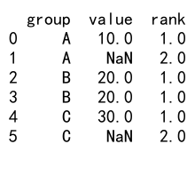
This example demonstrates how to handle NaN values and specify the correct ascending order when using pandas groupby rank.

Real-world Applications of Pandas GroupBy Rank

Pandas groupby rank has numerous real-world applications across various industries. Let’s explore some examples:

Finance: Portfolio Performance Analysis

import pandas as pd
import numpy as np

# Create a sample portfolio dataframe
np.random.seed(42)
df = pd.DataFrame({
    'date': pd.date_range(start='2023-01-01', periods=100, freq='D'),
    'stock': np.random.choice(['AAPL', 'GOOGL', 'MSFT', 'AMZN'], 100),
    'return': np.random.normal(0.001, 0.02, 100)
})

# Calculate cumulative returns
df['cumulative_return'] = df.groupby('stock')['return'].cumsum()

# Rank stocks based on cumulative returns
df['rank'] = df.groupby('date')['cumulative_return'].rank(ascending=False)

# Calculate average rank for each stock
avg_rank = df.groupby('stock')['rank'].mean().sort_values()

print(avg_rank)

Output:

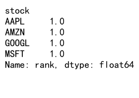
This example demonstrates how pandas groupby rank can be used to analyze and rank stock performance within a portfolio over time.

E-commerce: Customer Segmentation

import pandas as pd
import numpy as np

# Create a sample customer dataframe
np.random.seed(42)
df = pd.DataFrame({
    'customer_id': range(1000),
    'total_spend': np.random.exponential(500, 1000),
    'order_frequency': np.random.poisson(5, 1000),
    'category': np.random.choice(['Electronics', 'Clothing', 'Home', 'Books'], 1000)
})

# Calculate RFM (Recency, Frequency, Monetary) scores
df['spend_rank'] = df.groupby('category')['total_spend'].rank(pct=True)
df['frequency_rank'] = df.groupby('category')['order_frequency'].rank(pct=True)
df['rfm_score'] = (df['spend_rank'] + df['frequency_rank']) / 2

# Segment customers based on RFM score
df['segment'] = pd.qcut(df['rfm_score'], q=4, labels=['Bronze', 'Silver', 'Gold', 'Platinum'])

print(df.head(10))

Output:

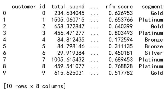
This example shows how pandas groupby rank can be used to calculate RFM (Recency, Frequency, Monetary) scores and segment customers based on their purchasing behavior within different product categories.

Conclusion

Pandas groupby rank is a powerful and versatile tool for data analysis and manipulation. By combining the groupby functionality with ranking operations, you can gain valuable insights into your data, identify patterns, and make data-driven decisions. Throughout this comprehensive guide, we’ve explored various aspects of pandas groupby rank, including:

1. Basic concepts and usage
2. Advanced techniques and applications
3. Handling ties and percentile ranking
4. Combining with other pandas operations
5. Performance optimization
6. Common pitfalls and how to avoid them
7. Real-world applications in finance and e-commerce

As you continue to work with pandas groupby rank, you’ll discover even more ways to leverage this powerful feature in your data analysis projects. Remember to experiment with different ranking methods, explore multi-level grouping, and combine groupby rank with other pandas operations to unlock the full potential of your data.

Best Practices for Using Pandas GroupBy Rank

To make the most of pandas groupby rank in your data analysis workflows, consider the following best practices:

1. Always specify the ranking method: Choose the appropriate method (e.g., ‘dense’, ‘min’, ‘max’) based on your specific requirements.

2. Handle missing values carefully: Use the na_option parameter to control how NaN values are treated in your rankings.

3. Use descriptive column names: When creating new columns for ranks, use clear and descriptive names to improve code readability.

4. Combine with other pandas functions: Leverage the full power of pandas by combining groupby rank with other operations like filtering, aggregation, and transformation.

5. Document your ranking logic: Clearly document the reasoning behind your ranking choices, especially for complex ranking scenarios.

Let’s see an example that incorporates these best practices:

import pandas as pd
import numpy as np

# Create a sample sales dataframe
np.random.seed(42)
df = pd.DataFrame({
    'date': pd.date_range(start='2023-01-01', periods=100, freq='D'),
    'product': np.random.choice(['A', 'B', 'C', 'D'], 100),
    'sales': np.random.normal(1000, 200, 100),
    'returns': np.random.randint(0, 10, 100)
})

# Calculate net sales
df['net_sales'] = df['sales'] - df['returns'] * 100

# Rank products by net sales within each date
df['daily_sales_rank'] = df.groupby('date')['net_sales'].rank(
    method='dense',
    ascending=False,
    na_option='bottom'
)

# Calculate average rank for each product
avg_rank = df.groupby('product')['daily_sales_rank'].mean().sort_values()

# Identify top-performing products
top_products = df[df['daily_sales_rank'] == 1]['product'].value_counts()

print("Average product ranks:")
print(avg_rank)
print("\nTop-performing products by day:")
print(top_products)

Output:

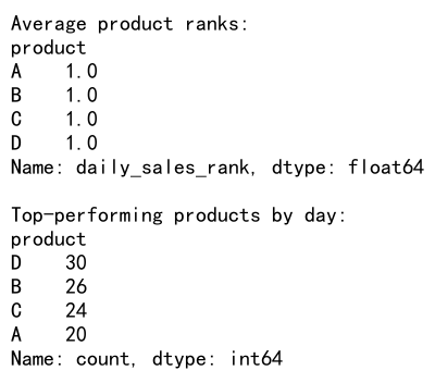
This example demonstrates best practices for using pandas groupby rank, including clear column naming, appropriate method selection, and combining ranking with other pandas operations for insightful analysis.

Advanced Pandas GroupBy Rank Techniques

As you become more comfortable with pandas groupby rank, you can explore more advanced techniques to enhance your data analysis capabilities. Here are some advanced techniques to consider:

Rolling Rankings

Rolling rankings allow you to calculate ranks within a moving window of data, which can be useful for time-series analysis:

import pandas as pd
import numpy as np

# Create a sample time-series dataframe
np.random.seed(42)
df = pd.DataFrame({
    'date': pd.date_range(start='2023-01-01', periods=100, freq='D'),
    'stock': np.random.choice(['AAPL', 'GOOGL', 'MSFT', 'AMZN'], 100),
    'return': np.random.normal(0.001, 0.02, 100)
})

# Sort the dataframe by date and stock
df = df.sort_values(['date', 'stock'])

# Calculate 7-day rolling return
df['rolling_return'] = df.groupby('stock')['return'].rolling(window=7).sum().reset_index(level=0, drop=True)

# Calculate rolling rank
df['rolling_rank'] = df.groupby('date')['rolling_return'].rank(ascending=False)

print(df.head(10))

Output:

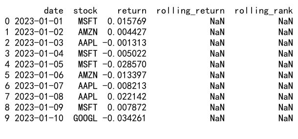
This example demonstrates how to calculate rolling rankings for stock returns, which can help identify trends in performance over time.

Weighted Rankings

In some cases, you may want to assign different weights to different factors when calculating ranks. Here’s an example of how to implement weighted rankings:

import pandas as pd
import numpy as np

# Create a sample student performance dataframe
np.random.seed(42)
df = pd.DataFrame({
    'student': [f'student_{i}' for i in range(100)],
    'exam_score': np.random.uniform(60, 100, 100),
    'project_score': np.random.uniform(70, 100, 100),
    'attendance': np.random.uniform(80, 100, 100)
})

# Define weights for each factor
weights = {
    'exam_score': 0.5,
    'project_score': 0.3,
    'attendance': 0.2
}

# Calculate weighted score
df['weighted_score'] = sum(df[col] * weight for col, weight in weights.items())

# Calculate weighted rank
df['weighted_rank'] = df['weighted_score'].rank(ascending=False, method='dense')

print(df.head(10))

Output:

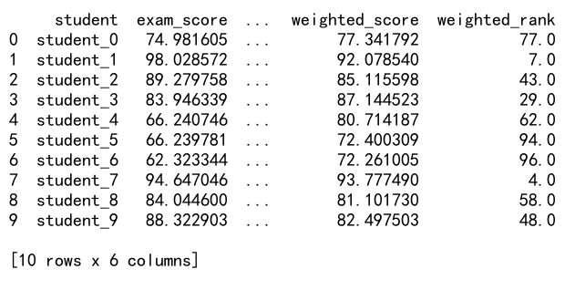
This example shows how to create a weighted ranking system for student performance, taking into account multiple factors with different levels of importance.

Integrating Pandas GroupBy Rank with Data Visualization

Visualizing the results of pandas groupby rank operations can provide valuable insights and make your analysis more accessible. Let’s explore some ways to integrate pandas groupby rank with data visualization libraries like matplotlib and seaborn:

import pandas as pd
import numpy as np
import matplotlib.pyplot as plt
import seaborn as sns

# Create a sample sales dataframe
np.random.seed(42)
df = pd.DataFrame({
    'product': np.repeat(['A', 'B', 'C', 'D', 'E'], 20),
    'region': np.random.choice(['North', 'South', 'East', 'West'], 100),
    'sales': np.random.normal(1000, 200, 100)
})

# Calculate sales rank within each region
df['sales_rank'] = df.groupby('region')['sales'].rank(ascending=False)

# Create a heatmap of sales ranks
pivot_df = df.pivot(index='product', columns='region', values='sales_rank')
plt.figure(figsize=(10, 6))
sns.heatmap(pivot_df, annot=True, cmap='YlGnBu', fmt='g')
plt.title('Sales Rank by Product and Region')
plt.show()

# Create a bar plot of average sales rank by product
avg_rank = df.groupby('product')['sales_rank'].mean().sort_values()
plt.figure(figsize=(10, 6))
avg_rank.plot(kind='bar')
plt.title('Average Sales Rank by Product')
plt.xlabel('Product')
plt.ylabel('Average Rank')
plt.show()

This example demonstrates how to create visualizations based on pandas groupby rank results, including a heatmap of sales ranks and a bar plot of average ranks by product.