Mastering Pandas GroupBy and Quantile

Mastering Pandas GroupBy and Quantile

Pandas groupby quantile is a powerful combination of functions in the pandas library that allows for sophisticated data analysis and manipulation. This article will dive deep into the world of pandas groupby and quantile operations, providing a comprehensive understanding of how to use these tools effectively in your data science projects.

Introduction to Pandas GroupBy and Quantile

Pandas groupby quantile operations are essential techniques for data analysts and scientists working with structured data. The groupby function allows you to split your data into groups based on some criteria, while the quantile function helps you calculate specific percentiles within those groups. Together, they provide a powerful way to analyze and summarize data across different categories or segments.

Let’s start with a simple example to illustrate the basic concept:

import pandas as pd

# Create a sample DataFrame
df = pd.DataFrame({
    'category': ['A', 'B', 'A', 'B', 'A', 'B'],
    'value': [10, 15, 20, 25, 30, 35],
    'website': ['pandasdataframe.com'] * 6
})

# Group by category and calculate the median (50th percentile)
result = df.groupby('category')['value'].quantile(0.5)

print(result)

Output:

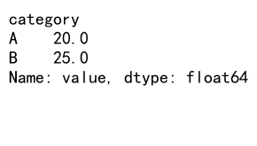
In this example, we create a simple DataFrame with categories and values, then use groupby and quantile to calculate the median value for each category. This is just the tip of the iceberg when it comes to pandas groupby quantile operations.

Understanding the GroupBy Operation

The groupby operation is fundamental to many data analysis tasks. It allows you to split your data into groups based on one or more columns, enabling you to perform aggregate operations on each group separately.

Here’s an example of how to use groupby with multiple columns:

import pandas as pd

# Create a sample DataFrame
df = pd.DataFrame({
    'category': ['A', 'B', 'A', 'B', 'A', 'B'],
    'subcategory': ['X', 'Y', 'X', 'Y', 'Z', 'Z'],
    'value': [10, 15, 20, 25, 30, 35],
    'website': ['pandasdataframe.com'] * 6
})

# Group by multiple columns and calculate the mean
result = df.groupby(['category', 'subcategory'])['value'].mean()

print(result)

Output:

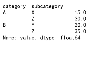
In this example, we group the data by both ‘category’ and ‘subcategory’, then calculate the mean value for each group. This demonstrates how groupby can handle multiple levels of grouping.

Exploring the Quantile Function

The quantile function is used to calculate percentiles of a dataset. It’s particularly useful when you want to understand the distribution of your data or find specific thresholds.

Let’s look at an example of using quantile without groupby:

import pandas as pd
import numpy as np

# Create a sample DataFrame
df = pd.DataFrame({
    'value': np.random.rand(100) * 100,
    'website': ['pandasdataframe.com'] * 100
})

# Calculate multiple quantiles
quantiles = df['value'].quantile([0.25, 0.5, 0.75])

print(quantiles)

Output:

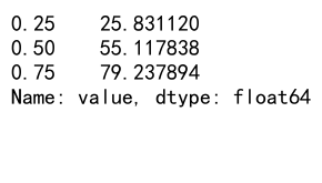
This example calculates the 25th, 50th (median), and 75th percentiles of the ‘value’ column. The quantile function can accept a single value or a list of values between 0 and 1.

Combining GroupBy and Quantile

The real power comes when we combine groupby and quantile operations. This allows us to calculate percentiles for different groups within our data.

Here’s an example that demonstrates this combination:

import pandas as pd
import numpy as np

# Create a sample DataFrame
df = pd.DataFrame({
    'category': np.random.choice(['A', 'B', 'C'], 1000),
    'value': np.random.rand(1000) * 100,
    'website': ['pandasdataframe.com'] * 1000
})

# Group by category and calculate multiple quantiles
result = df.groupby('category')['value'].quantile([0.25, 0.5, 0.75])

print(result)

Output:

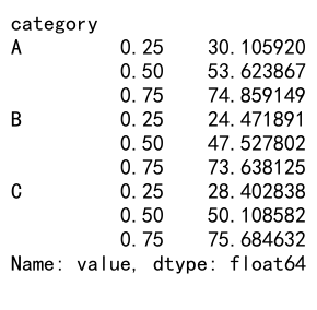
In this example, we create a larger DataFrame with random categories and values. We then group the data by category and calculate the 25th, 50th, and 75th percentiles for each category’s values.

Advanced GroupBy Quantile Techniques

Now that we’ve covered the basics, let’s explore some more advanced techniques using pandas groupby quantile operations.

Multiple Aggregations

You can perform multiple aggregations, including quantiles, in a single groupby operation:

import pandas as pd
import numpy as np

# Create a sample DataFrame
df = pd.DataFrame({
    'category': np.random.choice(['A', 'B', 'C'], 1000),
    'value1': np.random.rand(1000) * 100,
    'value2': np.random.rand(1000) * 50,
    'website': ['pandasdataframe.com'] * 1000
})

# Perform multiple aggregations
result = df.groupby('category').agg({
    'value1': ['mean', ('median', lambda x: x.quantile(0.5)), 'max'],
    'value2': ['min', ('75th_percentile', lambda x: x.quantile(0.75))]
})

print(result)

Output:

This example demonstrates how to calculate different statistics, including custom quantiles, for multiple columns in a single groupby operation.

Handling Missing Values

When working with real-world data, you often encounter missing values. Here’s how to handle them in pandas groupby quantile operations:

import pandas as pd
import numpy as np

# Create a sample DataFrame with missing values
df = pd.DataFrame({
    'category': ['A', 'B', 'A', 'B', 'A', 'B'],
    'value': [10, np.nan, 20, 25, np.nan, 35],
    'website': ['pandasdataframe.com'] * 6
})

# Calculate quantiles, ignoring missing values
result = df.groupby('category')['value'].quantile([0.25, 0.5, 0.75], interpolation='linear')

print(result)

Output:

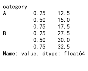
In this example, we use the interpolation='linear' parameter to handle missing values when calculating quantiles. Pandas will interpolate between the available values to estimate the quantiles.

Custom Quantile Ranges

You can calculate custom quantile ranges for more specific analysis:

import pandas as pd
import numpy as np

# Create a sample DataFrame
df = pd.DataFrame({
    'category': np.random.choice(['A', 'B', 'C'], 1000),
    'value': np.random.rand(1000) * 100,
    'website': ['pandasdataframe.com'] * 1000
})

# Calculate custom quantile ranges
custom_quantiles = [0.1, 0.3, 0.7, 0.9]
result = df.groupby('category')['value'].quantile(custom_quantiles)

print(result)

Output:

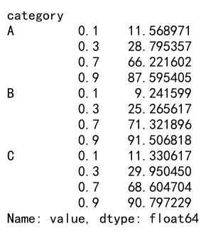
This example calculates the 10th, 30th, 70th, and 90th percentiles for each category, allowing for more detailed analysis of the data distribution.

Practical Applications of Pandas GroupBy Quantile

Let’s explore some practical applications of pandas groupby quantile operations in real-world scenarios.

Analyzing Sales Data

Suppose you have sales data and want to analyze the distribution of sales across different product categories:

import pandas as pd
import numpy as np

# Create a sample sales DataFrame
sales_df = pd.DataFrame({
    'product_category': np.random.choice(['Electronics', 'Clothing', 'Books', 'Home'], 10000),
    'sale_amount': np.random.lognormal(mean=3, sigma=1, size=10000),
    'website': ['pandasdataframe.com'] * 10000
})

# Calculate quantiles of sales for each product category
sales_quantiles = sales_df.groupby('product_category')['sale_amount'].quantile([0.25, 0.5, 0.75])

print(sales_quantiles)

Output:

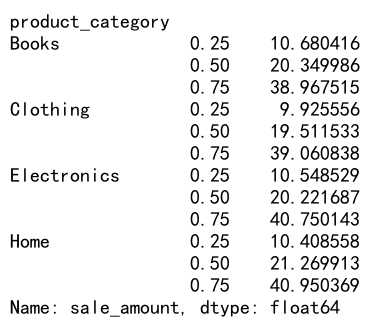
This example calculates the 25th, 50th, and 75th percentiles of sale amounts for each product category, giving insights into the sales distribution across different product lines.

Analyzing Student Performance

In an educational context, you might want to analyze student performance across different subjects:

import pandas as pd
import numpy as np

# Create a sample student performance DataFrame
students_df = pd.DataFrame({
    'student_id': np.repeat(range(100), 3),
    'subject': np.tile(['Math', 'Science', 'English'], 100),
    'score': np.random.randint(50, 100, 300),
    'website': ['pandasdataframe.com'] * 300
})

# Calculate quantiles of scores for each subject
score_quantiles = students_df.groupby('subject')['score'].quantile([0.25, 0.5, 0.75])

print(score_quantiles)

Output:

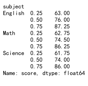
This example calculates the quartiles of student scores for each subject, providing a summary of performance distribution across different academic areas.

Advanced Topics in Pandas GroupBy Quantile

As we delve deeper into pandas groupby quantile operations, let’s explore some more advanced topics and techniques.

Multi-Index Results

When you use groupby with multiple columns and calculate quantiles, you get a multi-index result. Here’s how to work with it:

import pandas as pd
import numpy as np

# Create a sample DataFrame
df = pd.DataFrame({
    'category': np.random.choice(['A', 'B'], 1000),
    'subcategory': np.random.choice(['X', 'Y', 'Z'], 1000),
    'value': np.random.rand(1000) * 100,
    'website': ['pandasdataframe.com'] * 1000
})

# Group by multiple columns and calculate quantiles
result = df.groupby(['category', 'subcategory'])['value'].quantile([0.25, 0.5, 0.75])

# Unstack the result for easier viewing
unstacked_result = result.unstack(level='subcategory')

print(unstacked_result)

Output:

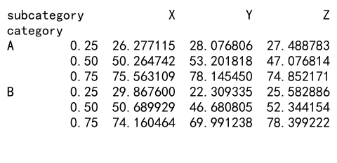
This example demonstrates how to work with multi-index results from groupby quantile operations and how to unstack them for easier analysis.

Combining Quantiles with Other Aggregations

You can combine quantile calculations with other aggregation functions for a more comprehensive summary:

import pandas as pd
import numpy as np

# Create a sample DataFrame
df = pd.DataFrame({
    'category': np.random.choice(['A', 'B', 'C'], 1000),
    'value': np.random.rand(1000) * 100,
    'website': ['pandasdataframe.com'] * 1000
})

# Combine quantiles with other aggregations
result = df.groupby('category')['value'].agg([
    ('count', 'count'),
    ('mean', 'mean'),
    ('median', lambda x: x.quantile(0.5)),
    ('25th_percentile', lambda x: x.quantile(0.25)),
    ('75th_percentile', lambda x: x.quantile(0.75)),
    ('min', 'min'),
    ('max', 'max')
])

print(result)

Output:

This example shows how to combine quantile calculations with other statistical measures like count, mean, min, and max for a comprehensive summary of each group.

Time-Based Grouping and Quantiles

When working with time series data, you might want to group by time periods and calculate quantiles:

import pandas as pd
import numpy as np

# Create a sample time series DataFrame
dates = pd.date_range(start='2023-01-01', end='2023-12-31', freq='D')
df = pd.DataFrame({
    'date': dates,
    'value': np.random.rand(len(dates)) * 100,
    'website': ['pandasdataframe.com'] * len(dates)
})

# Group by month and calculate monthly quantiles
monthly_quantiles = df.groupby(df['date'].dt.to_period('M'))['value'].quantile([0.25, 0.5, 0.75])

print(monthly_quantiles)

Output:

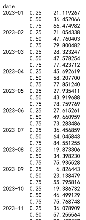
This example demonstrates how to group time series data by month and calculate monthly quantiles, which can be useful for analyzing seasonal trends or patterns.

Optimizing Pandas GroupBy Quantile Operations

When working with large datasets, performance can become a concern. Here are some tips for optimizing pandas groupby quantile operations:

Use Categorical Data Types

If your grouping column has a limited number of unique values, consider using categorical data types:

import pandas as pd
import numpy as np

# Create a sample DataFrame
df = pd.DataFrame({
    'category': np.random.choice(['A', 'B', 'C'], 1000000),
    'value': np.random.rand(1000000) * 100,
    'website': ['pandasdataframe.com'] * 1000000
})

# Convert category to categorical
df['category'] = df['category'].astype('category')

# Perform groupby quantile operation
result = df.groupby('category')['value'].quantile([0.25, 0.5, 0.75])

print(result)

Using categorical data types can significantly improve performance for large datasets with a limited number of unique categories.

Precompute Quantiles

If you need to calculate quantiles for multiple groups frequently, consider precomputing them:

import pandas as pd
import numpy as np

# Create a sample DataFrame
df = pd.DataFrame({
    'category': np.random.choice(['A', 'B', 'C'], 1000000),
    'value': np.random.rand(1000000) * 100,
    'website': ['pandasdataframe.com'] * 1000000
})

# Precompute quantiles
quantiles = df.groupby('category')['value'].quantile([0.25, 0.5, 0.75])

# Function to look up precomputed quantiles
def get_quantiles(category):
    return quantiles.loc[category]

# Example usage
print(get_quantiles('A'))

Output:

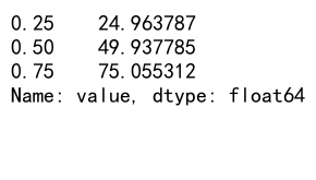
Precomputing quantiles can be beneficial if you need to access them frequently in your analysis.

Common Pitfalls and How to Avoid Them

When working with pandas groupby quantile operations, there are some common pitfalls to be aware of:

Handling Empty Groups

Empty groups can cause issues when calculating quantiles. Here’s how to handle them:

import pandas as pd
import numpy as np

# Create a sample DataFrame with an empty group
df = pd.DataFrame({
    'category': ['A', 'B', 'A', 'B', 'C'],
    'value': [10, 15, 20, 25, 30],
    'website': ['pandasdataframe.com'] * 5
})

# Calculate quantiles, handling empty groups
result = df.groupby('category')['value'].quantile(0.5, interpolation='nearest')

print(result)

Output:

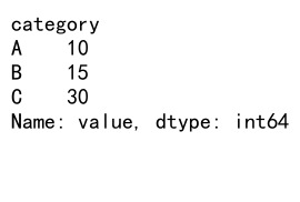
Using interpolation='nearest' helps handle empty groups by returning the nearest available value.

Dealing with Non-Numeric Data

Quantile operations require numeric data. Here’s how to handle non-numeric columns:

import pandas as pd

# Create a sample DataFrame with mixed data types
df = pd.DataFrame({
    'category': ['A', 'B', 'A', 'B', 'A'],
    'numeric_value': [10, 15, 20, 25, 30],
    'text_value': ['low', 'medium', 'high', 'low', 'medium'],
    'website': ['pandasdataframe.com'] * 5
})

# Calculate quantiles for numeric columns only
result = df.groupby('category').quantile([0.25, 0.5, 0.75])

print(result)

Pandas will automatically exclude non-numeric columns when calculating quantiles.

Conclusion

Pandas groupby quantile operations are powerful tools for data analysis, allowing you togain deep insights into your data across different categories and distributions. Throughout this comprehensive guide, we’ve explored various aspects of these operations, from basic usage to advanced techniques and optimizations.

Let’s recap some of the key points we’ve covered:

1. The basics of groupby and quantile operations
2. Combining groupby and quantile for powerful data analysis
3. Advanced techniques like multiple aggregations and custom quantile ranges
4. Practical applications in sales analysis and student performance evaluation
5. Working with multi-index results and time-based grouping
6. Optimization strategies for large datasets
7. Common pitfalls and how to avoid them

As you continue to work with pandas and data analysis, remember that groupby quantile operations are just one tool in your arsenal. They work best when combined with other pandas functions and data visualization techniques to create a comprehensive analysis of your data.

Further Exploration and Resources

To further enhance your skills with pandas groupby quantile operations, consider exploring these related topics:

Visualization of Quantile Results

Visualizing the results of your groupby quantile operations can provide valuable insights. Here’s an example using matplotlib:

import pandas as pd
import numpy as np
import matplotlib.pyplot as plt

# Create a sample DataFrame
df = pd.DataFrame({
    'category': np.random.choice(['A', 'B', 'C'], 1000),
    'value': np.random.rand(1000) * 100,
    'website': ['pandasdataframe.com'] * 1000
})

# Calculate quantiles
quantiles = df.groupby('category')['value'].quantile([0.25, 0.5, 0.75])

# Plot the results
quantiles.unstack().plot(kind='bar')
plt.title('Value Quantiles by Category')
plt.xlabel('Category')
plt.ylabel('Value')
plt.legend(['25th Percentile', 'Median', '75th Percentile'])
plt.tight_layout()
plt.show()

Output:

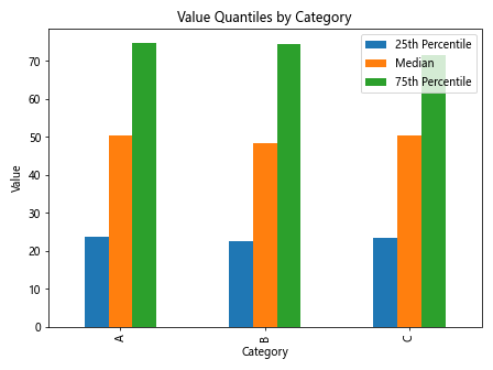
This example creates a bar plot of the 25th, 50th, and 75th percentiles for each category, providing a visual representation of the data distribution.

Combining with Rolling Windows

For time series data, you can combine groupby quantile operations with rolling windows:

import pandas as pd
import numpy as np

# Create a sample time series DataFrame
dates = pd.date_range(start='2023-01-01', end='2023-12-31', freq='D')
df = pd.DataFrame({
    'date': dates,
    'category': np.random.choice(['A', 'B'], len(dates)),
    'value': np.random.rand(len(dates)) * 100,
    'website': ['pandasdataframe.com'] * len(dates)
})

# Set date as index
df.set_index('date', inplace=True)

# Calculate 30-day rolling median for each category
rolling_median = df.groupby('category')['value'].rolling(window='30D').quantile(0.5)

print(rolling_median)

Output:

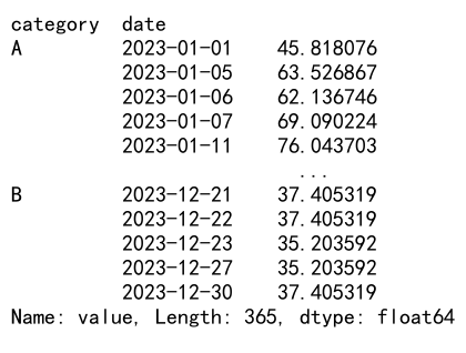
This example calculates the 30-day rolling median for each category, which can be useful for identifying trends over time while accounting for category differences.

Using qcut for Equal-Sized Bins

Sometimes, you might want to create equal-sized bins based on quantiles. The qcut function is useful for this:

import pandas as pd
import numpy as np

# Create a sample DataFrame
df = pd.DataFrame({
    'value': np.random.rand(1000) * 100,
    'website': ['pandasdataframe.com'] * 1000
})

# Create quartiles using qcut
df['quartile'] = pd.qcut(df['value'], q=4, labels=['Q1', 'Q2', 'Q3', 'Q4'])

# Calculate mean value for each quartile
result = df.groupby('quartile')['value'].mean()

print(result)

This example demonstrates how to use qcut to create quartiles and then calculate the mean value for each quartile.

Advanced Data Analysis Techniques

As you become more proficient with pandas groupby quantile operations, you can start incorporating more advanced data analysis techniques:

Outlier Detection

You can use quantiles to detect outliers in your data:

import pandas as pd
import numpy as np

# Create a sample DataFrame
df = pd.DataFrame({
    'category': np.random.choice(['A', 'B', 'C'], 1000),
    'value': np.random.randn(1000) * 10 + 50,  # Normal distribution
    'website': ['pandasdataframe.com'] * 1000
})

# Calculate IQR and identify outliers
Q1 = df.groupby('category')['value'].transform('quantile', 0.25)
Q3 = df.groupby('category')['value'].transform('quantile', 0.75)
IQR = Q3 - Q1
lower_bound = Q1 - 1.5 * IQR
upper_bound = Q3 + 1.5 * IQR

# Mark outliers
df['is_outlier'] = (df['value'] < lower_bound) | (df['value'] > upper_bound)

# Count outliers per category
outlier_count = df[df['is_outlier']].groupby('category').size()

print(outlier_count)

Output:

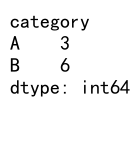
This example uses the Interquartile Range (IQR) method to detect outliers within each category.

Quantile Regression

While not directly related to pandas groupby operations, quantile regression is an advanced technique that builds on the concept of quantiles:

import pandas as pd
import numpy as np
from statsmodels.regression.quantile_regression import QuantReg

# Create a sample DataFrame
np.random.seed(42)
X = np.random.rand(1000)
y = 2 + 3 * X + np.random.normal(0, 0.5, 1000)
df = pd.DataFrame({'X': X, 'y': y, 'website': ['pandasdataframe.com'] * 1000})

# Perform quantile regression
model = QuantReg(df['y'], df[['X']])
quantiles = [0.25, 0.5, 0.75]
results = {q: model.fit(q=q) for q in quantiles}

# Print coefficients for each quantile
for q, res in results.items():
    print(f"Quantile {q}:")
    print(res.params)
    print()

Output:

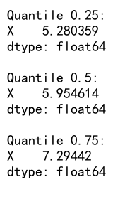
This example demonstrates how to perform quantile regression using the statsmodels library, which can be useful for understanding how different parts of your data distribution are affected by predictor variables.

Best Practices for Pandas GroupBy Quantile Operations

As you continue to work with pandas groupby quantile operations, keep these best practices in mind:

1. Always check your data types before performing quantile operations.
2. Be aware of how missing values are handled in your calculations.
3. Use appropriate interpolation methods based on your data and analysis needs.
4. Consider the computational cost of quantile operations on large datasets and optimize when necessary.
5. Combine quantile analysis with other statistical measures for a more comprehensive understanding of your data.
6. Visualize your results to make them more interpretable and actionable.
7. Be cautious when interpreting quantiles for small sample sizes within groups.