Mastering Pandas GroupBy with Index

Mastering Pandas GroupBy with Index

Pandas groupby index is a powerful feature in the pandas library that allows you to group data based on index values and perform aggregate operations on the resulting groups. This article will dive deep into the various aspects of using pandas groupby with index, providing detailed explanations and practical examples to help you master this essential data manipulation technique.

Understanding Pandas GroupBy Index

Pandas groupby index is a method that enables you to group data in a DataFrame based on the values in its index. This is particularly useful when you want to perform operations on subsets of your data that share common index values. By using pandas groupby index, you can efficiently analyze and transform your data in ways that would be difficult or time-consuming with other methods.

Let’s start with a simple example to illustrate the basic concept of pandas groupby index:

import pandas as pd

# Create a sample DataFrame
df = pd.DataFrame({
    'A': ['foo', 'bar', 'foo', 'bar', 'foo', 'bar'],
    'B': [1, 2, 3, 4, 5, 6]
}, index=['pandasdataframe.com', 'example.com', 'pandasdataframe.com', 'example.com', 'pandasdataframe.com', 'example.com'])

# Group by index and calculate the mean of column B
grouped = df.groupby(level=0)['B'].mean()

print(grouped)

Output:

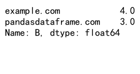
In this example, we create a DataFrame with two columns and an index containing two unique values. We then use pandas groupby index to group the data by the index values and calculate the mean of column B for each group.

Benefits of Using Pandas GroupBy Index

Using pandas groupby index offers several advantages when working with structured data:

1. Efficient data aggregation: Pandas groupby index allows you to quickly summarize large datasets based on common index values.

2. Flexible grouping: You can group data using single or multiple index levels, providing fine-grained control over your analysis.

3. Easy integration with other pandas functions: Pandas groupby index works seamlessly with other pandas operations, making it a versatile tool for data manipulation.

4. Improved performance: Grouping by index can be faster than grouping by columns, especially for large datasets.

Let’s explore these benefits with a more complex example:

import pandas as pd
import numpy as np

# Create a multi-index DataFrame
index = pd.MultiIndex.from_product([['pandasdataframe.com', 'example.com'], ['2021', '2022', '2023']], names=['website', 'year'])
df = pd.DataFrame({
    'visits': np.random.randint(1000, 10000, size=6),
    'revenue': np.random.uniform(100, 1000, size=6)
}, index=index)

# Group by the first index level and calculate multiple aggregations
grouped = df.groupby(level='website').agg({
    'visits': ['sum', 'mean'],
    'revenue': ['sum', 'mean']
})

print(grouped)

Output:

In this example, we create a multi-index DataFrame and use pandas groupby index to calculate multiple aggregations for each website. This demonstrates the flexibility and power of pandas groupby index when working with complex data structures.

Grouping by Single Index Level

When working with a single-level index, pandas groupby index allows you to group data based on the unique values in that index. This is particularly useful when you want to perform operations on subsets of your data that share common characteristics.

Here’s an example of grouping by a single index level:

import pandas as pd

# Create a sample DataFrame with a single-level index
df = pd.DataFrame({
    'product': ['A', 'B', 'A', 'B', 'A', 'B'],
    'sales': [100, 200, 150, 250, 180, 300]
}, index=['pandasdataframe.com', 'example.com', 'pandasdataframe.com', 'example.com', 'pandasdataframe.com', 'example.com'])

# Group by index and calculate total sales for each website
grouped = df.groupby(level=0)['sales'].sum()

print(grouped)

Output:

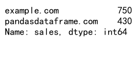
In this example, we group the data by the index (website) and calculate the total sales for each website. The resulting Series contains the sum of sales for each unique index value.

Grouping by Multiple Index Levels

Pandas groupby index becomes even more powerful when working with multi-index DataFrames. You can group data by one or more index levels, allowing for more complex and nuanced analyses.

Here’s an example of grouping by multiple index levels:

import pandas as pd
import numpy as np

# Create a multi-index DataFrame
index = pd.MultiIndex.from_product([['pandasdataframe.com', 'example.com'], ['2021', '2022', '2023'], ['Q1', 'Q2', 'Q3', 'Q4']], names=['website', 'year', 'quarter'])
df = pd.DataFrame({
    'revenue': np.random.uniform(1000, 10000, size=24),
    'expenses': np.random.uniform(500, 5000, size=24)
}, index=index)

# Group by website and year, then calculate the sum of revenue and expenses
grouped = df.groupby(level=['website', 'year']).sum()

print(grouped)

Output:

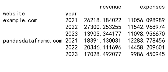
In this example, we create a multi-index DataFrame with three levels: website, year, and quarter. We then group the data by website and year, calculating the sum of revenue and expenses for each combination.

Applying Custom Functions with Pandas GroupBy Index

One of the most powerful features of pandas groupby index is the ability to apply custom functions to grouped data. This allows you to perform complex calculations or transformations on your data that go beyond simple aggregations.

Here’s an example of applying a custom function with pandas groupby index:

import pandas as pd
import numpy as np

# Create a sample DataFrame
df = pd.DataFrame({
    'category': ['A', 'B', 'A', 'B', 'A', 'B'],
    'value': [10, 20, 15, 25, 30, 35]
}, index=['pandasdataframe.com', 'example.com', 'pandasdataframe.com', 'example.com', 'pandasdataframe.com', 'example.com'])

# Define a custom function to calculate the percentage of total
def percent_of_total(group):
    return group / group.sum() * 100

# Apply the custom function to grouped data
grouped = df.groupby(level=0)['value'].transform(percent_of_total)

print(grouped)

Output:

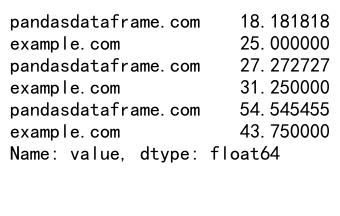
In this example, we define a custom function percent_of_total that calculates the percentage of the total for each group. We then apply this function to the grouped data using the transform method, which returns a Series with the same index as the original DataFrame.

Handling Missing Data in Pandas GroupBy Index

When working with real-world data, it’s common to encounter missing values. Pandas groupby index provides several options for handling missing data during grouping and aggregation operations.

Here’s an example of handling missing data with pandas groupby index:

import pandas as pd
import numpy as np

# Create a sample DataFrame with missing values
df = pd.DataFrame({
    'A': ['foo', 'bar', 'foo', 'bar', 'foo', 'bar'],
    'B': [1, 2, np.nan, 4, 5, np.nan]
}, index=['pandasdataframe.com', 'example.com', 'pandasdataframe.com', 'example.com', 'pandasdataframe.com', 'example.com'])

# Group by index and calculate the mean of column B, ignoring NaN values
grouped = df.groupby(level=0)['B'].mean(skipna=True)

print(grouped)

In this example, we create a DataFrame with missing values (NaN) in column B. When grouping and calculating the mean, we use the skipna=True parameter to ignore NaN values in the calculation.

Reshaping Data with Pandas GroupBy Index

Pandas groupby index can be used to reshape your data, allowing you to create new DataFrames with different structures based on your grouping criteria. This is particularly useful for pivoting data or creating summary tables.

Here’s an example of reshaping data with pandas groupby index:

import pandas as pd
import numpy as np

# Create a sample DataFrame
df = pd.DataFrame({
    'date': pd.date_range(start='2023-01-01', periods=6),
    'category': ['A', 'B', 'A', 'B', 'A', 'B'],
    'value': np.random.randint(1, 100, size=6)
})

# Set the index to date and category
df.set_index(['date', 'category'], inplace=True)

# Reshape the data to create a pivot table
reshaped = df.groupby(level=['date', 'category'])['value'].sum().unstack()

print(reshaped)

Output:

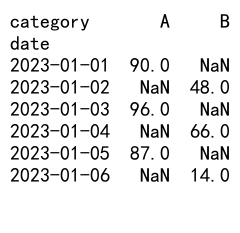
In this example, we create a DataFrame with a multi-index of date and category. We then use pandas groupby index to reshape the data into a pivot table, where each category becomes a column and the dates remain as the index.

Combining Pandas GroupBy Index with Other Operations

Pandas groupby index can be combined with other pandas operations to perform more complex data manipulations. This allows you to create powerful data processing pipelines that can handle a wide range of analytical tasks.

Here’s an example of combining pandas groupby index with other operations:

import pandas as pd
import numpy as np

# Create a sample DataFrame
df = pd.DataFrame({
    'A': ['foo', 'bar', 'foo', 'bar', 'foo', 'bar'],
    'B': np.random.randint(1, 100, size=6),
    'C': np.random.randint(1, 100, size=6)
}, index=['pandasdataframe.com', 'example.com', 'pandasdataframe.com', 'example.com', 'pandasdataframe.com', 'example.com'])

# Group by index, calculate the mean, and then filter the results
grouped = df.groupby(level=0).mean()
filtered = grouped[grouped['B'] > grouped['B'].mean()]

print(filtered)

In this example, we first group the data by index and calculate the mean for each group. We then filter the resulting DataFrame to show only the groups where the value in column B is greater than the overall mean of column B.

Performance Considerations for Pandas GroupBy Index

While pandas groupby index is a powerful tool, it’s important to consider performance when working with large datasets. Here are some tips to optimize your pandas groupby index operations:

1. Use appropriate data types: Ensure your index and columns have the correct data types to avoid unnecessary type conversions.
2. Limit the number of groups: Grouping by too many unique values can lead to memory issues and slow performance.
3. Use efficient aggregation functions: Some aggregation functions are faster than others. For example, sum() is generally faster than mean().
4. Consider using groupby().apply() for complex operations: For more complex operations, groupby().apply() can be more efficient than chaining multiple operations.

Here’s an example demonstrating some of these performance considerations:

import pandas as pd
import numpy as np

# Create a large DataFrame
n_rows = 1000000
df = pd.DataFrame({
    'A': np.random.choice(['foo', 'bar', 'baz'], size=n_rows),
    'B': np.random.randint(1, 100, size=n_rows),
    'C': np.random.uniform(0, 1, size=n_rows)
}, index=[f'pandasdataframe.com_{i}' for i in range(n_rows)])

# Efficient grouping and aggregation
grouped = df.groupby('A').agg({'B': 'sum', 'C': 'mean'})

print(grouped)

Output:

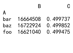
In this example, we create a large DataFrame with 1 million rows and perform an efficient grouping and aggregation operation. By using appropriate data types and efficient aggregation functions, we can process large datasets more quickly.

Advanced Techniques with Pandas GroupBy Index

As you become more comfortable with pandas groupby index, you can explore more advanced techniques to handle complex data analysis tasks. Here are some advanced techniques you can use:

1. Group-wise operations: Perform operations that depend on the entire group, not just individual elements.
2. Rolling window calculations: Apply rolling window functions to grouped data.
3. Grouping with categorical data: Use pandas’ categorical data type for more efficient grouping.
4. Custom aggregation functions: Create your own aggregation functions for unique analysis requirements.

Let’s explore an example of a group-wise operation using pandas groupby index:

import pandas as pd
import numpy as np

# Create a sample DataFrame
df = pd.DataFrame({
    'A': ['foo', 'bar', 'foo', 'bar', 'foo', 'bar'],
    'B': np.random.randint(1, 100, size=6),
    'C': np.random.uniform(0, 1, size=6)
}, index=['pandasdataframe.com', 'example.com', 'pandasdataframe.com', 'example.com', 'pandasdataframe.com', 'example.com'])

# Define a custom group-wise operation
def group_percentile(group):
    return group.rank(pct=True)

# Apply the group-wise operation
grouped = df.groupby(level=0).transform(group_percentile)

print(grouped)

Output:

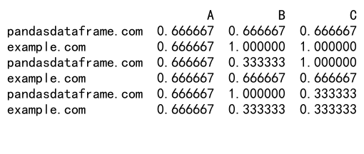
In this example, we define a custom group-wise operation that calculates the percentile rank of each value within its group. We then apply this operation to the grouped data using the transform method.

Handling Time Series Data with Pandas GroupBy Index

Pandas groupby index is particularly useful when working with time series data. You can use it to resample data, calculate rolling statistics, or perform time-based aggregations.

Here’s an example of using pandas groupby index with time series data:

import pandas as pd
import numpy as np

# Create a sample time series DataFrame
dates = pd.date_range(start='2023-01-01', end='2023-12-31', freq='D')
df = pd.DataFrame({
    'value': np.random.randint(1, 100, size=len(dates))
}, index=dates)

# Resample the data to monthly frequency and calculate the mean
monthly = df.groupby(pd.Grouper(freq='M'))['value'].mean()

print(monthly)

In this example, we create a daily time series DataFrame and use pandas groupby index with pd.Grouper to resample the data to a monthly frequency, calculating the mean value for each month.

Visualizing Grouped Data

After performing groupby operations, it’s often helpful to visualize the results. Pandas integrates well with various plotting libraries, making it easy to create visualizations of your grouped data.

Here’s an example of visualizing grouped data using matplotlib:

import pandas as pd
import numpy as np
import matplotlib.pyplot as plt

# Create a sample DataFrame
df = pd.DataFrame({
    'category': ['A', 'B', 'C', 'A', 'B', 'C'],
    'value': np.random.randint(1, 100, size=6)
}, index=['pandasdataframe.com', 'example.com', 'pandasdataframe.com', 'example.com', 'pandasdataframe.com', 'example.com'])

# Group by category and calculate the mean
grouped = df.groupby('category')['value'].mean()

# Create a bar plot
grouped.plot(kind='bar')
plt.title('Mean Value by Category')
plt.xlabel('Category')
plt.ylabel('Mean Value')
plt.show()

Output:

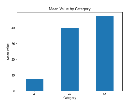
In this example, we group the data by category, calculate the mean value for each category, and then create a bar plot to visualize the results.

Conclusion

Pandas groupby index is a powerful and versatile tool for data analysis and manipulation. By mastering this feature, you can efficiently process and analyze large datasets, perform complex aggregations, and gain valuable insights from your data. Whether you’re working with simple tabular data or complex multi-index structures, pandas groupby index provides theflexibility and functionality you need to tackle a wide range of data analysis tasks.

Throughout this article, we’ve explored various aspects of pandas groupby index, including:

• Basic concepts and benefits
• Grouping by single and multiple index levels
• Applying custom functions
• Handling missing data
• Reshaping data
• Combining with other pandas operations
• Performance considerations
• Advanced techniques
• Working with time series data
• Visualizing grouped data

By incorporating these techniques into your data analysis workflow, you can significantly enhance your ability to extract meaningful insights from your data.

Best Practices for Using Pandas GroupBy Index

To make the most of pandas groupby index, consider the following best practices:

1. Choose appropriate grouping keys: Select index levels that are relevant to your analysis and provide meaningful groupings.

2. Use efficient aggregation functions: Opt for built-in aggregation functions when possible, as they are optimized for performance.

3. Handle missing data appropriately: Decide how to treat missing values based on your specific use case and data requirements.

4. Leverage multi-index capabilities: Take advantage of multi-index grouping for more complex analyses.

5. Combine with other pandas functions: Integrate groupby operations with other pandas functions to create powerful data processing pipelines.

6. Profile and optimize performance: Monitor the performance of your groupby operations, especially when working with large datasets.

7. Document your code: Clearly comment your groupby operations to explain the purpose and logic behind each step.

Let’s look at an example that incorporates some of these best practices:

import pandas as pd
import numpy as np

# Create a sample multi-index DataFrame
index = pd.MultiIndex.from_product([['pandasdataframe.com', 'example.com'], ['2021', '2022', '2023'], ['Q1', 'Q2', 'Q3', 'Q4']], names=['website', 'year', 'quarter'])
df = pd.DataFrame({
    'revenue': np.random.uniform(1000, 10000, size=24),
    'expenses': np.random.uniform(500, 5000, size=24),
    'customers': np.random.randint(100, 1000, size=24)
}, index=index)

# Define a custom aggregation function
def profit_margin(group):
    return (group['revenue'].sum() - group['expenses'].sum()) / group['revenue'].sum()

# Perform groupby operation with multiple aggregations
result = df.groupby(level=['website', 'year']).agg({
    'revenue': 'sum',
    'expenses': 'sum',
    'customers': 'mean'
})

# Add a custom aggregation
result['profit_margin'] = df.groupby(level=['website', 'year']).apply(profit_margin)

print(result)

Output:

In this example, we demonstrate several best practices:

1. We use a multi-index DataFrame to represent hierarchical data.
2. We choose appropriate grouping keys (website and year) for our analysis.
3. We use efficient built-in aggregation functions (sum and mean) where possible.
4. We define a custom aggregation function (profit_margin) for a more complex calculation.
5. We combine multiple aggregations in a single operation for efficiency.

Common Pitfalls and How to Avoid Them

While pandas groupby index is a powerful tool, there are some common pitfalls that you should be aware of:

1. Forgetting to reset the index: After groupby operations, the result often has a multi-index. Remember to reset the index if you need a flat DataFrame.

2. Ignoring data types: Grouping by columns with inappropriate data types can lead to unexpected results or poor performance.

3. Not handling missing data: Failing to account for missing data can skew your results or cause errors in your analysis.

4. Overcomplicating groupby operations: Sometimes, simpler approaches using other pandas functions might be more appropriate.

5. Memory issues with large datasets: Grouping very large datasets can consume a lot of memory. Consider using chunking or other optimization techniques for big data.

Let’s look at an example that demonstrates how to avoid some of these pitfalls:

import pandas as pd
import numpy as np

# Create a sample DataFrame with mixed data types and missing values
df = pd.DataFrame({
    'A': ['foo', 'bar', 'foo', 'bar', 'foo', 'bar'],
    'B': [1, 2, 3, 4, 5, 6],
    'C': ['a', 'b', 'c', 'd', np.nan, 'f'],
    'D': [1.1, 2.2, np.nan, 4.4, 5.5, 6.6]
}, index=['pandasdataframe.com', 'example.com', 'pandasdataframe.com', 'example.com', 'pandasdataframe.com', 'example.com'])

# Ensure appropriate data types
df['B'] = df['B'].astype('int32')
df['D'] = df['D'].astype('float32')

# Handle missing data
df['C'] = df['C'].fillna('unknown')
df['D'] = df['D'].fillna(df['D'].mean())

# Perform groupby operation
grouped = df.groupby(level=0).agg({
    'B': 'sum',
    'C': lambda x: ', '.join(x.unique()),
    'D': 'mean'
})

# Reset index if needed
grouped_flat = grouped.reset_index()

print(grouped)
print("\nFlat DataFrame:")
print(grouped_flat)

Output:

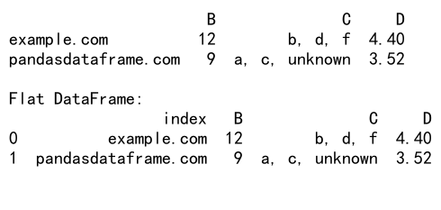
In this example, we address several common pitfalls:

1. We ensure appropriate data types for columns B and D.
2. We handle missing data in columns C and D using appropriate methods.
3. We use a mix of built-in and custom aggregation functions based on the data type and analysis requirements.
4. We demonstrate how to reset the index to create a flat DataFrame if needed.

Advanced Use Cases for Pandas GroupBy Index

As you become more proficient with pandas groupby index, you can tackle more complex data analysis tasks. Here are some advanced use cases:

1. Time-based rolling calculations
2. Group-wise regression analysis
3. Custom group transformations
4. Hierarchical indexing and analysis

Let’s explore an example of a time-based rolling calculation using pandas groupby index:

import pandas as pd
import numpy as np

# Create a sample time series DataFrame
dates = pd.date_range(start='2023-01-01', end='2023-12-31', freq='D')
df = pd.DataFrame({
    'value': np.random.randint(1, 100, size=len(dates)),
    'category': np.random.choice(['A', 'B', 'C'], size=len(dates))
}, index=dates)

# Perform a 7-day rolling average for each category
rolling_avg = df.groupby('category')['value'].rolling(window=7).mean().reset_index()

# Pivot the result for easier visualization
result = rolling_avg.pivot(index='level_1', columns='category', values='value')

print(result)

Output:

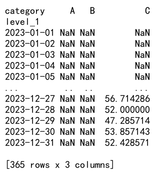
In this advanced example, we perform a 7-day rolling average calculation for each category in our time series data. This type of analysis is common in financial and economic data analysis, where you might want to smooth out short-term fluctuations and highlight longer-term trends.

Integrating Pandas GroupBy Index with Other Libraries

Pandas groupby index can be integrated with other popular data science libraries to extend its capabilities. Here are some examples:

1. Scikit-learn for machine learning tasks
2. Statsmodels for statistical modeling
3. Plotly for interactive visualizations

Let’s look at an example that combines pandas groupby index with scikit-learn for a simple machine learning task:

import pandas as pd
import numpy as np
from sklearn.preprocessing import StandardScaler
from sklearn.model_selection import train_test_split
from sklearn.linear_model import LogisticRegression
from sklearn.metrics import accuracy_score

# Create a sample DataFrame
df = pd.DataFrame({
    'feature1': np.random.randint(1, 100, size=1000),
    'feature2': np.random.uniform(0, 1, size=1000),
    'category': np.random.choice(['A', 'B', 'C'], size=1000)
}, index=[f'pandasdataframe.com_{i}' for i in range(1000)])

# Group by category and calculate mean and std for feature1
grouped_stats = df.groupby('category')['feature1'].agg(['mean', 'std'])

# Merge the grouped stats back to the original DataFrame
df = df.merge(grouped_stats, left_on='category', right_index=True)

# Create new features based on the grouped statistics
df['feature1_normalized'] = (df['feature1'] - df['mean']) / df['std']

# Prepare the data for machine learning
X = df[['feature1_normalized', 'feature2']]
y = (df['category'] == 'A').astype(int)  # Binary classification: A vs. not A

# Split the data into training and testing sets
X_train, X_test, y_train, y_test = train_test_split(X, y, test_size=0.2, random_state=42)

# Scale the features
scaler = StandardScaler()
X_train_scaled = scaler.fit_transform(X_train)
X_test_scaled = scaler.transform(X_test)

# Train a logistic regression model
model = LogisticRegression()
model.fit(X_train_scaled, y_train)

# Make predictions and calculate accuracy
y_pred = model.predict(X_test_scaled)
accuracy = accuracy_score(y_test, y_pred)

print(f"Model accuracy: {accuracy:.2f}")

Output:

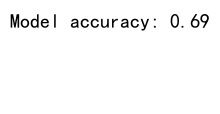
In this example, we use pandas groupby index to calculate group-specific statistics (mean and standard deviation) for a feature. We then use these statistics to create a new normalized feature. This preprocessed data is then used to train a simple logistic regression model using scikit-learn.