Mastering Pandas GroupBy with Bins

Mastering Pandas GroupBy with Bins

Pandas groupby bins is a powerful feature in the pandas library that allows you to group data into bins or intervals for analysis. This technique is particularly useful when dealing with continuous data that you want to categorize into discrete groups. In this comprehensive guide, we’ll explore the ins and outs of pandas groupby bins, providing detailed explanations and practical examples to help you master this essential data analysis tool.

Understanding Pandas GroupBy Bins

Pandas groupby bins is a combination of two powerful pandas features: groupby and cut/qcut. The groupby function allows you to group data based on specific criteria, while cut and qcut functions enable you to create bins or intervals from continuous data. When used together, these features provide a flexible way to analyze and summarize data across different categories or ranges.

Let’s start with a simple example to illustrate the concept of pandas groupby bins:

import pandas as pd
import numpy as np

# Create a sample DataFrame
df = pd.DataFrame({
    'value': np.random.randint(0, 100, 1000),
    'category': ['A', 'B', 'C'] * 333 + ['A']
})

# Define bins
bins = [0, 25, 50, 75, 100]
labels = ['Low', 'Medium-Low', 'Medium-High', 'High']

# Create a new column with binned values
df['value_group'] = pd.cut(df['value'], bins=bins, labels=labels, include_lowest=True)

# Group by the binned values and calculate the mean
result = df.groupby('value_group')['value'].mean()

print("pandasdataframe.com - Result:")
print(result)

Output:

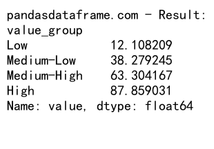
In this example, we create a sample DataFrame with random values and categories. We then use pandas groupby bins to group the ‘value’ column into four bins: Low (0-25), Medium-Low (26-50), Medium-High (51-75), and High (76-100). Finally, we calculate the mean value for each bin.

Benefits of Using Pandas GroupBy Bins

Pandas groupby bins offers several advantages for data analysis:

1. Simplifies complex data: By grouping continuous data into bins, you can simplify large datasets and make them easier to analyze and visualize.

2. Reveals patterns: Binning data can help uncover patterns or trends that might not be apparent in the raw data.

3. Facilitates comparisons: Grouping data into bins allows for easier comparisons between different ranges or categories.

4. Enhances statistical analysis: Binned data can be used for various statistical analyses, such as frequency distributions or cross-tabulations.

5. Improves data visualization: Binned data is often easier to visualize using charts and graphs, making it more accessible to stakeholders.

Creating Bins with Pandas Cut and Qcut

Before we dive deeper into pandas groupby bins, let’s explore the two main functions used for creating bins: cut and qcut.

Pandas Cut

The pd.cut() function is used to bin values into discrete intervals. It’s particularly useful when you want to specify the bin edges manually.

import pandas as pd
import numpy as np

# Create a sample Series
s = pd.Series(np.random.randint(0, 100, 1000))

# Create bins using cut
bins = [0, 25, 50, 75, 100]
labels = ['Low', 'Medium-Low', 'Medium-High', 'High']
binned_data = pd.cut(s, bins=bins, labels=labels, include_lowest=True)

print("pandasdataframe.com - Binned data:")
print(binned_data.value_counts())

Output:

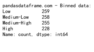
In this example, we use pd.cut() to bin a series of random numbers into four categories. The ‘bins’ parameter specifies the bin edges, and ‘labels’ provides names for each bin.

Pandas Qcut

The pd.qcut() function is used to create bins with equal frequencies. This is useful when you want to divide your data into quantiles.

import pandas as pd
import numpy as np

# Create a sample Series
s = pd.Series(np.random.randint(0, 100, 1000))

# Create bins using qcut
binned_data = pd.qcut(s, q=4, labels=['Q1', 'Q2', 'Q3', 'Q4'])

print("pandasdataframe.com - Binned data:")
print(binned_data.value_counts())

Output:

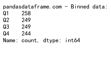
In this example, we use pd.qcut() to divide the data into four equal-sized bins (quartiles). The ‘q’ parameter specifies the number of quantiles.

Advanced Techniques with Pandas GroupBy Bins

Now that we’ve covered the basics, let’s explore some more advanced techniques using pandas groupby bins.

Customizing Bin Edges and Labels

You can customize bin edges and labels to suit your specific needs:

import pandas as pd
import numpy as np

# Create a sample DataFrame
df = pd.DataFrame({
    'age': np.random.randint(0, 100, 1000),
    'income': np.random.randint(20000, 150000, 1000)
})

# Define custom bins and labels
age_bins = [0, 18, 30, 50, 65, 100]
age_labels = ['Child', 'Young Adult', 'Adult', 'Middle-aged', 'Senior']
income_bins = [0, 30000, 60000, 100000, 150000]
income_labels = ['Low', 'Medium', 'High', 'Very High']

# Create binned columns
df['age_group'] = pd.cut(df['age'], bins=age_bins, labels=age_labels, include_lowest=True)
df['income_group'] = pd.cut(df['income'], bins=income_bins, labels=income_labels, include_lowest=True)

# Group by age and income groups
result = df.groupby(['age_group', 'income_group']).size().unstack(fill_value=0)

print("pandasdataframe.com - Result:")
print(result)

Output:

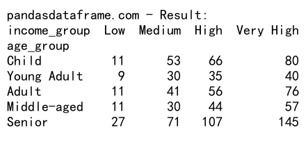
This example demonstrates how to create custom bins for both age and income, and then use pandas groupby bins to create a cross-tabulation of the results.

Using Pandas GroupBy Bins with Aggregation Functions

You can combine pandas groupby bins with various aggregation functions to perform more complex analyses:

import pandas as pd
import numpy as np

# Create a sample DataFrame
df = pd.DataFrame({
    'value': np.random.randint(0, 100, 1000),
    'category': ['A', 'B', 'C'] * 333 + ['A']
})

# Define bins
bins = [0, 25, 50, 75, 100]
labels = ['Low', 'Medium-Low', 'Medium-High', 'High']

# Create a new column with binned values
df['value_group'] = pd.cut(df['value'], bins=bins, labels=labels, include_lowest=True)

# Group by the binned values and calculate multiple aggregations
result = df.groupby('value_group').agg({
    'value': ['mean', 'median', 'std', 'count'],
    'category': lambda x: x.value_counts().index[0]
})

print("pandasdataframe.com - Result:")
print(result)

Output:

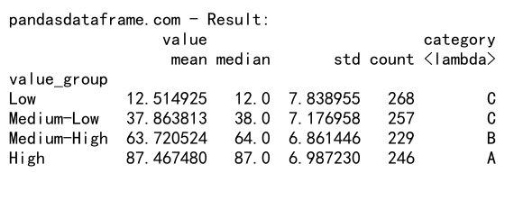
In this example, we use pandas groupby bins to calculate multiple aggregations for each bin, including mean, median, standard deviation, count, and the most common category.

Handling Datetime Data with Pandas GroupBy Bins

Pandas groupby bins can also be used with datetime data:

import pandas as pd
import numpy as np

# Create a sample DataFrame with datetime data
dates = pd.date_range(start='2023-01-01', end='2023-12-31', freq='D')
df = pd.DataFrame({
    'date': dates,
    'value': np.random.randint(0, 100, len(dates))
})

# Define bins for months
df['month'] = df['date'].dt.to_period('M')

# Group by month and calculate statistics
result = df.groupby('month').agg({
    'value': ['mean', 'median', 'min', 'max']
})

print("pandasdataframe.com - Result:")
print(result)

Output:

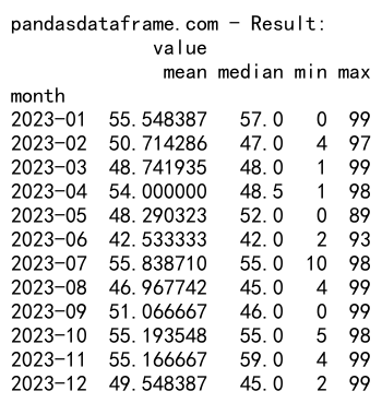
This example shows how to use pandas groupby bins with datetime data to analyze values by month.

Visualizing Pandas GroupBy Bins Results

Visualizing the results of pandas groupby bins can help in understanding patterns and trends in your data. Here’s an example using matplotlib:

import pandas as pd
import numpy as np
import matplotlib.pyplot as plt

# Create a sample DataFrame
df = pd.DataFrame({
    'value': np.random.randint(0, 100, 1000),
    'category': ['A', 'B', 'C'] * 333 + ['A']
})

# Define bins
bins = [0, 25, 50, 75, 100]
labels = ['Low', 'Medium-Low', 'Medium-High', 'High']

# Create a new column with binned values
df['value_group'] = pd.cut(df['value'], bins=bins, labels=labels, include_lowest=True)

# Group by the binned values and calculate the mean
result = df.groupby('value_group')['value'].mean()

# Create a bar plot
plt.figure(figsize=(10, 6))
result.plot(kind='bar')
plt.title('Average Value by Group')
plt.xlabel('Value Group')
plt.ylabel('Average Value')
plt.xticks(rotation=45)
plt.tight_layout()
plt.savefig('pandasdataframe.com_groupby_bins_plot.png')
plt.close()

print("pandasdataframe.com - Plot saved as 'pandasdataframe.com_groupby_bins_plot.png'")

This example creates a bar plot of the average value for each bin, providing a visual representation of the pandas groupby bins results.

Handling Missing Values in Pandas GroupBy Bins

When working with real-world data, you may encounter missing values. Here’s how to handle them using pandas groupby bins:

import pandas as pd
import numpy as np

# Create a sample DataFrame with missing values
df = pd.DataFrame({
    'value': np.random.randint(0, 100, 1000),
    'category': ['A', 'B', 'C'] * 333 + ['A']
})
df.loc[np.random.choice(df.index, 100), 'value'] = np.nan

# Define bins
bins = [0, 25, 50, 75, 100]
labels = ['Low', 'Medium-Low', 'Medium-High', 'High']

# Create a new column with binned values, handling missing values
df['value_group'] = pd.cut(df['value'], bins=bins, labels=labels, include_lowest=True)

# Group by the binned values and calculate statistics
result = df.groupby('value_group').agg({
    'value': ['count', 'mean', 'median'],
    'category': lambda x: x.value_counts().index[0]
})

print("pandasdataframe.com - Result:")
print(result)

Output:

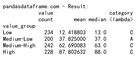
In this example, we introduce missing values to the DataFrame and show how pandas groupby bins handles them when creating bins and calculating statistics.

Combining Pandas GroupBy Bins with Other GroupBy Operations

You can combine pandas groupby bins with other groupby operations for more complex analyses:

import pandas as pd
import numpy as np

# Create a sample DataFrame
df = pd.DataFrame({
    'value': np.random.randint(0, 100, 1000),
    'category': ['A', 'B', 'C'] * 333 + ['A'],
    'region': np.random.choice(['North', 'South', 'East', 'West'], 1000)
})

# Define bins
bins = [0, 25, 50, 75, 100]
labels = ['Low', 'Medium-Low', 'Medium-High', 'High']

# Create a new column with binned values
df['value_group'] = pd.cut(df['value'], bins=bins, labels=labels, include_lowest=True)

# Group by multiple columns including the binned values
result = df.groupby(['region', 'value_group', 'category']).agg({
    'value': ['count', 'mean', 'median']
})

print("pandasdataframe.com - Result:")
print(result)

Output:

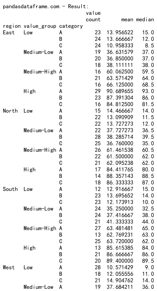
This example demonstrates how to combine pandas groupby bins with other groupby operations, such as grouping by region and category.

Using Pandas GroupBy Bins for Time Series Analysis

Pandas groupby bins can be particularly useful for time series analysis. Here’s an example of how to use it with financial data:

import pandas as pd
import numpy as np
import yfinance as yf

# Download stock data
stock_data = yf.download('AAPL', start='2022-01-01', end='2023-12-31')

# Calculate daily returns
stock_data['Daily_Return'] = stock_data['Close'].pct_change()

# Define bins for returns
bins = [-np.inf, -0.02, -0.01, 0, 0.01, 0.02, np.inf]
labels = ['Large Loss', 'Small Loss', 'Minimal Loss', 'Minimal Gain', 'Small Gain', 'Large Gain']

# Create a new column with binned returns
stock_data['Return_Group'] = pd.cut(stock_data['Daily_Return'], bins=bins, labels=labels)

# Group by return group and calculate statistics
result = stock_data.groupby('Return_Group').agg({
    'Daily_Return': ['count', 'mean'],
    'Volume': 'mean'
})

print("pandasdataframe.com - Result:")
print(result)

This example shows how to use pandas groupby bins to analyze stock returns and trading volume based on different return categories.

Optimizing Performance with Pandas GroupBy Bins

When working with large datasets, optimizing the performance of pandas groupby bins operations becomes crucial. Here are some tips to improve efficiency:

1. Use categorical data types for binned columns:

import pandas as pd
import numpy as np

# Create a large sample DataFrame
df = pd.DataFrame({
    'value': np.random.randint(0, 100, 1000000),
    'category': np.random.choice(['A', 'B', 'C'], 1000000)
})

# Define bins
bins = [0, 25, 50, 75, 100]
labels = ['Low', 'Medium-Low', 'Medium-High', 'High']

# Create a new column with binned values as categorical
df['value_group'] = pd.Categorical(pd.cut(df['value'], bins=bins, labels=labels, include_lowest=True))

# Group by the binned values and calculate statistics
result = df.groupby('value_group').agg({
    'value': ['count', 'mean', 'median'],
    'category': lambda x: x.value_counts().index[0]
})

print("pandasdataframe.com - Result:")
print(result)

Output:

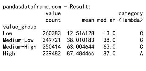
Using categorical data types for binned columns can significantly improve memory usage and performance, especially for large datasets.

2. Use numba for custom aggregation functions:

import pandas as pd
import numpy as np
from numba import jit

@jit(nopython=True)
def custom_agg(x):
    return np.mean(x) * np.median(x)

# Create a large sample DataFrame
df = pd.DataFrame({
    'value': np.random.randint(0, 100, 1000000),
    'category': np.random.choice(['A', 'B', 'C'], 1000000)
})

# Define bins
bins = [0, 25, 50, 75, 100]
labels = ['Low', 'Medium-Low', 'Medium-High', 'High']

# Create a new column with binned values
df['value_group'] = pd.cut(df['value'], bins=bins, labels=labels, include_lowest=True)

# Group by the binned values and calculate statistics using numba
result = df.groupby('value_group')['value'].agg(custom_agg)

print("pandasdataframe.com - Result:")
print(result)

Using numba to compile custom aggregation functions can significantly speed up complex calculations when using pandas groupby bins.

Advanced Applications of Pandas GroupBy Bins

Let’s explore some advanced applications of pandas groupby bins to showcase its versatility in data analysis.

Analyzing Customer Behavior

Pandas groupby bins can be used to analyze customer behavior based on various metrics:

import pandas as pd
import numpy as np

# Create a sample customer DataFrame
customers = pd.DataFrame({
    'customer_id': range(1000),
    'total_spend': np.random.randint(0, 10000, 1000),
    'age': np.random.randint(18, 80, 1000),
    'loyalty_years': np.random.randint(0, 10, 1000)
})

# Define bins for spending and age
spend_bins = [0, 1000, 2500, 5000, 10000]
spend_labels = ['Low', 'Medium', 'High', 'VIP']
age_bins = [18, 30, 45, 60, 80]
age_labels = ['Young', 'Adult', 'Middle-aged', 'Senior']

# Create binned columns
customers['spend_group'] = pd.cut(customers['total_spend'], bins=spend_bins, labels=spend_labels, include_lowest=True)
customers['age_group'] = pd.cut(customers['age'], bins=age_bins, labels=age_labels, include_lowest=True)

# Analyze customer segments
result = customers.groupby(['spend_group', 'age_group']).agg({
    'customer_id': 'count',
    'total_spend': 'mean',
    'loyalty_years': 'mean'
}).reset_index()

print("pandasdataframe.com - Customer Segment Analysis:")
print(result)

Output:

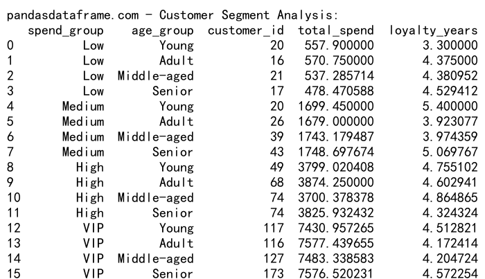
This example demonstrates how to use pandas groupby bins to segment customers based on their spending habits and age, providing insights into different customer groups.

Analyzing Environmental Data

Pandas groupby bins can be useful for analyzing environmental data, such as temperature readings:

import pandas as pd
import numpy as np

# Create a sample temperature DataFrame
temperatures = pd.DataFrame({
    'date': pd.date_range(start='2023-01-01', end='2023-12-31', freq='D'),
    'temperature': np.random.normal(15, 10, 365),
    'location': np.random.choice(['City A', 'City B', 'City C'], 365)
})

# Define temperature bins
temp_bins = [-np.inf, 0, 10, 20, 30, np.inf]
temp_labels = ['Freezing', 'Cold', 'Mild', 'Warm', 'Hot']

# Create binned temperature column
temperatures['temp_group'] = pd.cut(temperatures['temperature'], bins=temp_bins, labels=temp_labels)

# Analyze temperature distribution by location and month
temperatures['month'] = temperatures['date'].dt.to_period('M')
result = temperatures.groupby(['location', 'month', 'temp_group']).size().unstack(fill_value=0)

print("pandasdataframe.com - Temperature Distribution Analysis:")
print(result)

Output:

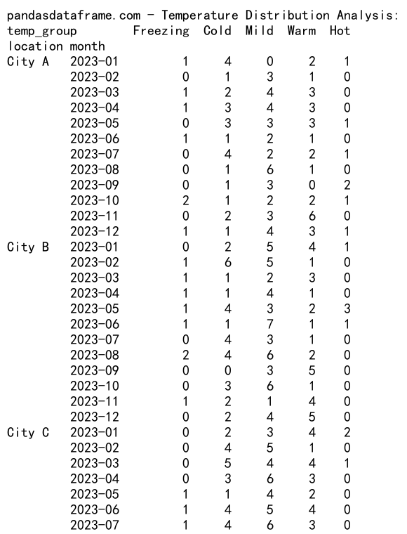
This example shows how to use pandas groupby bins to analyze temperature distributions across different locations and months.

Combining Pandas GroupBy Bins with Machine Learning

Pandas groupby bins can be a valuable tool in preparing data for machine learning models. Here’s an example of how to use it in a preprocessing pipeline:

import pandas as pd
import numpy as np
from sklearn.model_selection import train_test_split
from sklearn.preprocessing import StandardScaler
from sklearn.ensemble import RandomForestClassifier
from sklearn.metrics import accuracy_score

# Create a sample dataset
df = pd.DataFrame({
    'age': np.random.randint(18, 80, 1000),
    'income': np.random.randint(20000, 150000, 1000),
    'credit_score': np.random.randint(300, 850, 1000),
    'default': np.random.choice([0, 1], 1000, p=[0.9, 0.1])
})

# Define bins for continuous variables
age_bins = [18, 30, 45, 60, 80]
income_bins = [0, 30000, 60000, 100000, 150000]
credit_bins = [300, 500, 650, 750, 850]

# Create binned columns
df['age_group'] = pd.cut(df['age'], bins=age_bins, labels=['Young', 'Adult', 'Middle-aged', 'Senior'], include_lowest=True)
df['income_group'] = pd.cut(df['income'], bins=income_bins, labels=['Low', 'Medium', 'High', 'Very High'], include_lowest=True)
df['credit_group'] = pd.cut(df['credit_score'], bins=credit_bins, labels=['Poor', 'Fair', 'Good', 'Excellent'], include_lowest=True)

# Convert categorical variables to dummy variables
df_encoded = pd.get_dummies(df, columns=['age_group', 'income_group', 'credit_group'])

# Prepare features and target
X = df_encoded.drop(['default', 'age', 'income', 'credit_score'], axis=1)
y = df_encoded['default']

# Split the data
X_train, X_test, y_train, y_test = train_test_split(X, y, test_size=0.2, random_state=42)

# Scale the features
scaler = StandardScaler()
X_train_scaled = scaler.fit_transform(X_train)
X_test_scaled = scaler.transform(X_test)

# Train a Random Forest model
rf_model = RandomForestClassifier(n_estimators=100, random_state=42)
rf_model.fit(X_train_scaled, y_train)

# Make predictions and calculate accuracy
y_pred = rf_model.predict(X_test_scaled)
accuracy = accuracy_score(y_test, y_pred)

print("pandasdataframe.com - Model Accuracy:", accuracy)

Output:

This example demonstrates how to use pandas groupby bins to preprocess continuous variables into categorical bins, which can be useful for certain machine learning models.

Conclusion

Pandas groupby bins is a powerful and versatile tool for data analysis and preprocessing. By allowing you to group continuous data into meaningful categories, it enables more insightful analysis and can improve the performance of machine learning models. Throughout this comprehensive guide, we’ve explored various aspects of pandas groupby bins, including:

1. Basic concepts and usage
2. Advanced techniques and customization
3. Handling different data types, including datetime data
4. Visualizing results
5. Dealing with missing values
6. Combining with other groupby operations
7. Time series analysis
8. Performance optimization
9. Advanced applications in customer analysis and environmental data
10. Integration with machine learning workflows