Comprehensive Guide to Pandas GroupBy Agg Count All
Pandas groupby agg count all is a powerful combination of functions in the pandas library that allows for efficient data aggregation and analysis. This article will delve deep into the intricacies of using pandas groupby, agg, count, and all functions together to perform complex data operations. We’ll explore various scenarios where these functions can be applied and provide numerous examples to illustrate their usage.
Understanding Pandas GroupBy
Pandas groupby is a fundamental operation in data analysis that allows you to split your data into groups based on some criteria. When combined with aggregation functions like agg and count, it becomes a powerful tool for summarizing and analyzing data.
Let’s start with a simple example of using pandas groupby:
import pandas as pd

# Create a sample DataFrame
df = pd.DataFrame({
    'Name': ['John', 'Emma', 'John', 'Emma', 'Mike'],
    'Age': [25, 30, 25, 30, 35],
    'City': ['New York', 'London', 'New York', 'Paris', 'Tokyo'],
    'Salary': [50000, 60000, 55000, 65000, 70000]
})

# Group by 'Name' and calculate the mean salary
result = df.groupby('Name')['Salary'].mean()

print("Result from pandasdataframe.com:")
print(result)
Output:
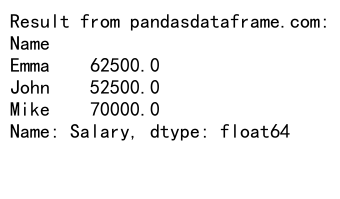
In this example, we group the DataFrame by the ‘Name’ column and calculate the mean salary for each person. The groupby operation splits the data into groups based on unique names, and then the mean function is applied to the ‘Salary’ column for each group.
Exploring the Agg Function
The agg function in pandas is a versatile tool that allows you to apply multiple aggregation functions to your grouped data. It’s particularly useful when you want to perform different operations on different columns within the same groupby operation.
Here’s an example demonstrating the use of agg:
import pandas as pd

# Create a sample DataFrame
df = pd.DataFrame({
    'Name': ['John', 'Emma', 'John', 'Emma', 'Mike'],
    'Age': [25, 30, 25, 30, 35],
    'City': ['New York', 'London', 'New York', 'Paris', 'Tokyo'],
    'Salary': [50000, 60000, 55000, 65000, 70000]
})

# Group by 'Name' and apply multiple aggregation functions
result = df.groupby('Name').agg({
    'Age': 'mean',
    'Salary': ['min', 'max', 'mean']
})

print("Result from pandasdataframe.com:")
print(result)
Output:
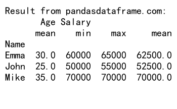
In this example, we group the data by ‘Name’ and then apply different aggregation functions to different columns. We calculate the mean age and the minimum, maximum, and mean salary for each person.
Utilizing the Count Function
The count function is another useful aggregation method that can be combined with groupby. It allows you to count the number of non-null values in each group.
Here’s an example of using count with groupby:
import pandas as pd

# Create a sample DataFrame
df = pd.DataFrame({
    'Name': ['John', 'Emma', 'John', 'Emma', 'Mike', 'John'],
    'Age': [25, 30, 25, 30, 35, None],
    'City': ['New York', 'London', 'New York', 'Paris', 'Tokyo', 'Berlin'],
    'Salary': [50000, 60000, 55000, 65000, 70000, None]
})

# Group by 'Name' and count non-null values
result = df.groupby('Name').count()

print("Result from pandasdataframe.com:")
print(result)
Output:
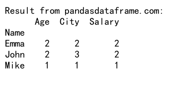
In this example, we group the data by ‘Name’ and count the number of non-null values for each column within each group. Note that the count function excludes NaN values from the count.
The All Function in Pandas
The all function in pandas is a boolean aggregation function that returns True if all elements in a group are True (or truthy). It’s particularly useful when you want to check if a certain condition holds for all members of a group.
Here’s an example of using all with groupby:
import pandas as pd

# Create a sample DataFrame
df = pd.DataFrame({
    'Name': ['John', 'Emma', 'John', 'Emma', 'Mike'],
    'Age': [25, 30, 25, 30, 35],
    'City': ['New York', 'London', 'New York', 'Paris', 'Tokyo'],
    'Salary': [50000, 60000, 55000, 65000, 70000]
})

# Check if all salaries in each group are above 40000
result = df.groupby('Name')['Salary'].agg(lambda x: (x > 40000).all())

print("Result from pandasdataframe.com:")
print(result)
Output:
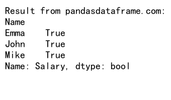
In this example, we group the data by ‘Name’ and then check if all salaries for each person are above 40000. The all function returns True for each group where the condition is met for all members of that group.
Combining GroupBy, Agg, Count, and All
Now that we’ve explored each of these functions individually, let’s see how we can combine them to perform more complex data operations.
Here’s an example that uses all of these functions together:
import pandas as pd

# Create a sample DataFrame
df = pd.DataFrame({
    'Name': ['John', 'Emma', 'John', 'Emma', 'Mike', 'John'],
    'Age': [25, 30, 25, 30, 35, None],
    'City': ['New York', 'London', 'New York', 'Paris', 'Tokyo', 'Berlin'],
    'Salary': [50000, 60000, 55000, 65000, 70000, None]
})

# Perform complex aggregation
result = df.groupby('Name').agg({
    'Age': ['count', 'mean', lambda x: x.notnull().all()],
    'Salary': ['count', 'min', 'max', 'mean', lambda x: (x > 50000).all()]
})

print("Result from pandasdataframe.com:")
print(result)
Output:

In this example, we’re performing a complex aggregation on our DataFrame. We group by ‘Name’ and then:
– For ‘Age’, we count the non-null values, calculate the mean, and check if all values are non-null.
– For ‘Salary’, we count the non-null values, find the minimum and maximum, calculate the mean, and check if all salaries are above 50000.
This demonstrates how we can combine groupby, agg, count, and all to perform sophisticated data analysis in a single operation.
Advanced GroupBy Techniques
Let’s explore some more advanced techniques using pandas groupby agg count all.
Multiple Column Grouping
You can group by multiple columns to create more specific groups:
import pandas as pd

# Create a sample DataFrame
df = pd.DataFrame({
    'Name': ['John', 'Emma', 'John', 'Emma', 'Mike', 'John'],
    'Department': ['Sales', 'HR', 'Sales', 'HR', 'IT', 'IT'],
    'Age': [25, 30, 25, 30, 35, 28],
    'Salary': [50000, 60000, 55000, 65000, 70000, 58000]
})

# Group by multiple columns
result = df.groupby(['Name', 'Department']).agg({
    'Age': ['mean', 'count'],
    'Salary': ['min', 'max', 'mean']
})

print("Result from pandasdataframe.com:")
print(result)
Output:
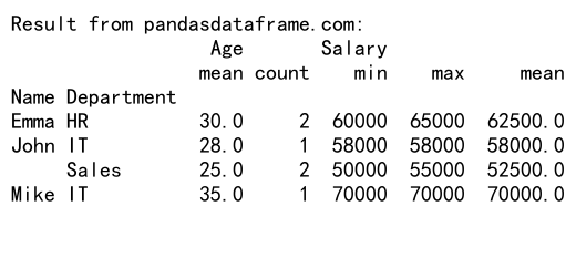
In this example, we group by both ‘Name’ and ‘Department’, allowing us to analyze data for each person in each department separately.
Using Named Aggregations
Pandas allows you to name your aggregations, which can make your results more readable:
import pandas as pd

# Create a sample DataFrame
df = pd.DataFrame({
    'Name': ['John', 'Emma', 'John', 'Emma', 'Mike', 'John'],
    'Age': [25, 30, 25, 30, 35, 28],
    'Salary': [50000, 60000, 55000, 65000, 70000, 58000]
})

# Use named aggregations
result = df.groupby('Name').agg(
    mean_age=('Age', 'mean'),
    min_salary=('Salary', 'min'),
    max_salary=('Salary', 'max')
)

print("Result from pandasdataframe.com:")
print(result)
Output:
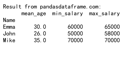
This approach gives clear names to each aggregation, making the resulting DataFrame easier to understand and work with.
Filtering Groups
You can use the filter method to keep only groups that satisfy a certain condition:
import pandas as pd

# Create a sample DataFrame
df = pd.DataFrame({
    'Name': ['John', 'Emma', 'John', 'Emma', 'Mike', 'John'],
    'Age': [25, 30, 25, 30, 35, 28],
    'Salary': [50000, 60000, 55000, 65000, 70000, 58000]
})

# Filter groups where the mean salary is above 60000
result = df.groupby('Name').filter(lambda x: x['Salary'].mean() > 60000)

print("Result from pandasdataframe.com:")
print(result)
Output:
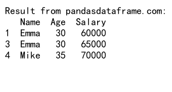
This example filters out groups (in this case, names) where the mean salary is not above 60000.
Handling Missing Data in GroupBy Operations
When working with real-world data, you’ll often encounter missing values. Let’s explore how pandas groupby agg count all handles missing data and how you can control this behavior.
Excluding Missing Data
By default, most aggregation functions in pandas exclude missing data:
import pandas as pd
import numpy as np

# Create a sample DataFrame with missing data
df = pd.DataFrame({
    'Name': ['John', 'Emma', 'John', 'Emma', 'Mike', 'John'],
    'Age': [25, 30, 25, np.nan, 35, 28],
    'Salary': [50000, 60000, 55000, 65000, np.nan, 58000]
})

# Perform aggregation
result = df.groupby('Name').agg({
    'Age': ['count', 'mean'],
    'Salary': ['count', 'mean']
})

print("Result from pandasdataframe.com:")
print(result)
Output:
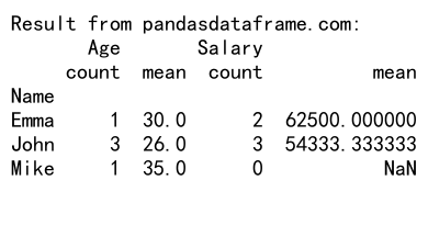
In this example, you’ll notice that the count and mean calculations automatically exclude NaN values.
Including Missing Data
If you want to include missing data in your calculations, you can use specific functions or modify existing ones:
import pandas as pd
import numpy as np

# Create a sample DataFrame with missing data
df = pd.DataFrame({
    'Name': ['John', 'Emma', 'John', 'Emma', 'Mike', 'John'],
    'Age': [25, 30, 25, np.nan, 35, 28],
    'Salary': [50000, 60000, 55000, 65000, np.nan, 58000]
})

# Include NaN values in count and mean
result = df.groupby('Name').agg({
    'Age': [('count_all', 'size'), ('mean_with_nan', lambda x: x.mean(skipna=False))],
    'Salary': [('count_all', 'size'), ('mean_with_nan', lambda x: x.mean(skipna=False))]
})

print("Result from pandasdataframe.com:")
print(result)
Output:
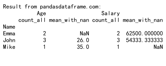
In this example, we use ‘size’ instead of ‘count’ to include NaN values in the count, and we use a custom lambda function for mean that doesn’t skip NaN values.
Time-Based Grouping with Pandas
Pandas is particularly powerful when working with time series data. Let’s explore how we can use pandas groupby agg count all with time-based data.
Grouping by Time Periods
You can group time series data by various time periods:
import pandas as pd
import numpy as np

# Create a sample DataFrame with date index
dates = pd.date_range('2023-01-01', periods=100, freq='D')
df = pd.DataFrame({
    'Date': dates,
    'Value': np.random.randn(100)
})

# Group by month and calculate statistics
result = df.groupby(df['Date'].dt.to_period('M')).agg({
    'Value': ['count', 'mean', 'std', 'min', 'max']
})

print("Result from pandasdataframe.com:")
print(result)
Output:
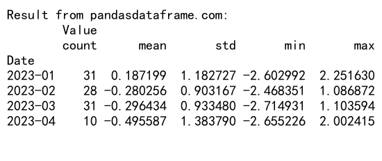
In this example, we group our data by month and calculate various statistics for each month.
Rolling Window Calculations
You can also perform rolling window calculations with groupby:
import pandas as pd
import numpy as np

# Create a sample DataFrame with date index
dates = pd.date_range('2023-01-01', periods=100, freq='D')
df = pd.DataFrame({
    'Date': dates,
    'Value': np.random.randn(100)
})

# Perform 7-day rolling average
df['7_day_avg'] = df.groupby(df['Date'].dt.to_period('M'))['Value'].transform(lambda x: x.rolling(7).mean())

print("Result from pandasdataframe.com:")
print(df.head(10))
Output:
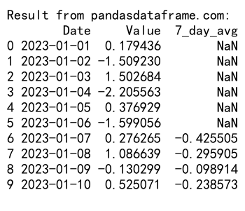
This example calculates a 7-day rolling average for each month separately.
Handling Categorical Data with GroupBy
Categorical data is common in many datasets. Let’s see how we can use pandas groupby agg count all with categorical data.
Handling Unused Categories
By default, unused categories are dropped in groupby operations. You can change this behavior:
import pandas as pd

# Create a sample DataFrame with categorical data
df = pd.DataFrame({
    'Category': ['A', 'B', 'A', 'C', 'B', 'A'],
    'Value': [10, 20, 15, 25, 30, 5]
})

# Convert 'Category' to categorical type with an unused category
df['Category'] = pd.Categorical(df['Category'], categories=['A', 'B', 'C', 'D'])

# Group by category and calculate statistics, including unused categories
result = df.groupby('Category', observed=False).agg({
    'Value': ['count', 'mean', 'min', 'max']
})

print("Result from pandasdataframe.com:")
print(result)
Output:
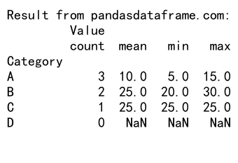
In this example, we include the unused category ‘D’ in our results by setting observed=False in the groupby operation.
Advanced Aggregation Techniques
Let’s explore some more advanced aggregation techniques using pandas groupby agg count all.
Custom Aggregation Functions
You can define your own aggregation functions to use with groupby:
import pandas as pd
import numpy as np

# Create a sample DataFrame
df = pd.DataFrame({
    'Name': ['John', 'Emma','John', 'Emma', 'Mike', 'John'],
    'Age': [25, 30, 25, 30, 35, 28],
    'Salary': [50000, 60000, 55000, 65000, 70000, 58000]
})

# Define a custom aggregation function
def salary_range(x):
    return x.max() - x.min()

# Use the custom function in aggregation
result = df.groupby('Name').agg({
    'Age': ['mean', 'std'],
    'Salary': ['mean', salary_range]
})

print("Result from pandasdataframe.com:")
print(result)
Output:
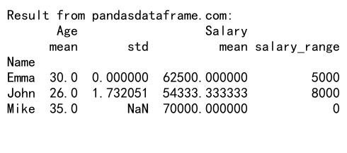
In this example, we define a custom function salary_range that calculates the range of salaries, and use it alongside built-in aggregation functions.
Aggregating with Conditional Logic
You can use conditional logic within your aggregations:
import pandas as pd

# Create a sample DataFrame
df = pd.DataFrame({
    'Name': ['John', 'Emma', 'John', 'Emma', 'Mike', 'John'],
    'Age': [25, 30, 25, 30, 35, 28],
    'Salary': [50000, 60000, 55000, 65000, 70000, 58000]
})

# Aggregate with conditional logic
result = df.groupby('Name').agg({
    'Age': 'mean',
    'Salary': [
        'mean',
        ('high_salary_count', lambda x: (x > 60000).sum()),
        ('low_salary_count', lambda x: (x <= 60000).sum())
    ]
})

print("Result from pandasdataframe.com:")
print(result)
Output:
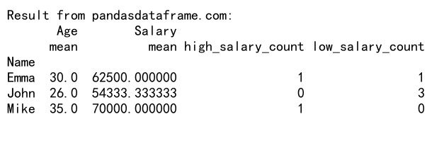
This example counts the number of high salaries (>60000) and low salaries (<=60000) for each person, alongside calculating the mean age and salary.
Handling Multi-Index Results
GroupBy operations often result in multi-index DataFrames. Let’s explore how to work with these:
Flattening Multi-Index Columns
import pandas as pd

# Create a sample DataFrame
df = pd.DataFrame({
    'Name': ['John', 'Emma', 'John', 'Emma', 'Mike', 'John'],
    'Age': [25, 30, 25, 30, 35, 28],
    'Salary': [50000, 60000, 55000, 65000, 70000, 58000]
})

# Perform aggregation resulting in multi-index columns
result = df.groupby('Name').agg({
    'Age': ['mean', 'std'],
    'Salary': ['mean', 'min', 'max']
})

# Flatten the multi-index columns
result.columns = ['_'.join(col).strip() for col in result.columns.values]

print("Result from pandasdataframe.com:")
print(result)
Output:

This example shows how to flatten multi-index columns into a single level for easier access.
Selecting from Multi-Index Results
import pandas as pd

# Create a sample DataFrame
df = pd.DataFrame({
    'Name': ['John', 'Emma', 'John', 'Emma', 'Mike', 'John'],
    'Age': [25, 30, 25, 30, 35, 28],
    'Salary': [50000, 60000, 55000, 65000, 70000, 58000]
})

# Perform aggregation resulting in multi-index columns
result = df.groupby('Name').agg({
    'Age': ['mean', 'std'],
    'Salary': ['mean', 'min', 'max']
})

# Select specific columns
age_mean = result['Age']['mean']
salary_max = result['Salary']['max']

print("Result from pandasdataframe.com:")
print("Mean Age:")
print(age_mean)
print("\nMax Salary:")
print(salary_max)
Output:
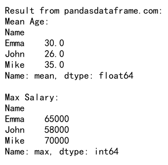
This example demonstrates how to select specific columns from a multi-index result.
Conclusion
Pandas groupby agg count all is a powerful combination of functions that allows for complex data analysis and aggregation. Throughout this article, we’ve explored various aspects of these functions, from basic usage to advanced techniques and optimizations.
We’ve seen how to:
– Use groupby to split data into groups
– Apply multiple aggregation functions with agg
– Count non-null values with count
– Check conditions across groups with all
– Handle missing data in groupby operations
– Work with time-based and categorical data
– Optimize groupby operations for large datasets
– Handle multi-index results
By mastering these techniques, you’ll be well-equipped to tackle a wide range of data analysis tasks efficiently and effectively. Remember that pandas is a versatile library, and there’s often more than one way to achieve a particular result. Experiment with different approaches to find the one that works best for your specific use case.
 Pandas Dataframe